
kff - Kalman Filter Framework
This framework functions as a Kalman filter, an extended Kalman filter, and an iterated extended Kalman filter with options for sequential updates, Joseph's form for numerically stable covariance updates, consider parameters (Schmidt-Kalman filter), and gain customization.
Interfaces
Simplest interface: the options struct contains the constants and
function handles, so that all other inputs are the inputs which change
from sample to sample:
[x_k, P_k] = kff(t_km1, t_k, x_km1, P_km1, z_k, options);where t_km1 is the time at sample k-1, t_k is the current time,
x_km1 is the prior estimate, P_km1 is the prior covariance, z_k is
the current measurement, and x_k and P_k are the updated forms.
The options input above comes from kffoptions. More on this below.
If there's an input vector, u_km1, we can pass that in too:
[x_k, P_k] = kff(t_km1, t_k, x_km1, P_km1, u_km1, z_k, options);Alternately, using an options structure isn't necessary. We can pass in the functions, Jacobians, and covariance matrices directly.
[x_k, P_k] = kff( ...
    t_km1, t_k, x_km1, P_km1, u_km1, z_k, ... % Signals
    f, F_km1, Q_km1, ...                      % Prediction
    h, H_k, R_k);                             % Observation
In the above, each of the inputs corresponding F_km1, Q_km1, H_k,
and R_k can, instead of being the matrix itself, be a function handle
that calculates the appropriate matrix. This is useful, e.g., for
iterated filters, which may need to calculate H_k and R_k multiple
times internally with slightly different values. See below for a
discussion of their interfaces.
Consider covariance can be added to either of the above forms directly.
[x_k, P_k, P_xc_k] = kff( ...
    t_km1, t_k, x_km1, P_km1, P_xc_km1, u_km1, z_k, options);
[x_k, P_k, P_xc_k] = kff( ...
    t_km1, dt, ...                          % Times
    x_km1, P_km1, P_xc_km1, u_km1, z_k, ... % Signals
    f, F_km1, F_c_km1, Q_km1, ...           % Prediction
    h, H_k, H_c_k, R_k, ...                 % Observation
    P_cc, ...                               % Consider covariance
    [options])                              % Additional options
where P_xc is the covariance between the state and consider parameters,
F_c_km1 and H_c_k are the Jacobians of the propagation and
observation functions wrt the consider parameters, and P_cc is the
consider covariance matrix.
Suppose that not all measurements are updated at the same time. We can
indicate this with an updates vector. This will have the same number of
elements as the measurement vector and will be true for the indices that
correspond to new measurements available on this sample. For instance, if
the second and third elements of a 3-element measurement vector are new,
the updates would be [false; true; true].
[x_k, P_k, P_xc_k] = kff(t_km1, t_k, x_km1, P_km1, P_xc_km1, ...
                         u_km1, z_k, updates, options);
Here are all unique possible input combinations (dropping subscripts for legibility):
kff(x, P, z, opt)
kff(x, P, u, z, opt)
kff(t, t, x, P, z, opt)
kff(t, t, x, P, u, z, opt)
kff(t, t, x, P, Pxc, u, z, opt)
kff(t, t, x, P, Pxc, u, z, upd, opt)
kff(x, P, z, f, F, Q, h, H, R, opt)
kff(x, P, u, z, f, F, Q, h, H, R)
kff(x, P, u, z, f, F, Q, h, H, R, opt)
kff(t, t, x, P, z, f, F, Q, h, H, R)
kff(t, t, x, P, z, f, F, Q, h, H, R, opt)
kff(t, t, x, P, u, z, f, F, Q, h, H, R)
kff(t, t, x, P, u, z, f, F, Q, h, H, R, opt)
kff(t, t, x, P, u, z, upd, f, F, Q, h, H, R)
kff(t, t, x, P, u, z, upd, f, F, Q, h, H, R, opt)
kff(x, P, Pxc, u, z, f, F, Fc, Q, h, H, Hc, R, Pc)
kff(x, P, Pxc, u, z, f, F, Fc, Q, h, H, Hc, R, Pc, opt)
kff(t, t, x, P, Pxc, z, f, F, Fc, Q, h, H, Hc, R, Pc)
kff(t, t, x, P, Pxc, z, upd, f, F, Fc, Q, h, H, Hc, R, Pc, opt)
kff(t, t, x, P, Pxc, u, z, f, F, Fc, Q, h, H, Hc, R, Pc)
kff(t, t, x, P, Pxc, u, z, f, F, Fc, Q, h, H, Hc, R, Pc, opt)
kff(t, t, x, P, Pxc, u, z, upd, f, F, Fc, Q, h, H, Hc, R, Pc)
kff(t, t, x, P, Pxc, u, z, upd, f, F, Fc, Q, h, H, Hc, R, Pc, opt)
Finally, the innovation vector and innovation covariance can both be output as well. These are useful when checking that the innovation is sufficiently "white" -- uncorrelated with itself from sample to sample.
[x_k, P_k, P_xc_k, y_k, S_k] = kff(...)Here's the whole interface. Note that you can leave things you don't
need, such as P_cc and P_xc) empty ([]). Any arguments after the
final options structure will be treated as option-value pairs (see
below).
[x, P, P_xc, y_k, S_k] = kff( ...
    t_km1, t_k, ...                           % Times
    x, P, P_xc, ...                           % State and covariances
    u_km1, z_k, updates, ...                  % Input and measurement
    f, F_km1_fcn, F_c_km1_fcn, Q_km1_fcn, ... % Propagation stuff
    h, H_k_fcn, H_c_k_fcn, R_k_fcn, ...       % Observatoin stuff
    P_cc, ...                                 % Consider covariance
    options, ...                              % kffoptions structure
    (etc.));                                  % Option-value pairs
Inputs
t_km1 | Time at sample k-1 |
|---|---|
t_k | Time at sample k |
x_km1 | Estimate of state at k-1 conditioned on observations at k-1, \(x_{k-1|k-1}\) |
P_km1 | Estimate covariance at k-1 |
P_xc_km1 | Covariance of state with considered parameters at k-1 |
u_km1 | Inputs vector at k-1 |
z_k | Observation vector at k |
updates | Array of booleans indicating which sensor groups have new
updates to incorporate into the estimate at sample k
(1-by- |
f | Function returning updated state at |
F_km1_fcn | The Jacobian of |
F_c_km1_fcn | The Jacobian of |
Q_km1_fcn | The process noise covariance matrix at |
h | Function returning the observations at |
H_k_fcn | The Jacobian of |
H_c_k_fcn | The Jacobian of |
R_k_fcn | The measurement noise covariance matrix at Optionally, for sequential updates, which require a
diagonal |
P_cc | Consider covariance (usually constant) |
options | Options structure from |
(etc.) | Option-value pairs (see below) |
Outputs
x_k | Updated state estimate at k |
|---|---|
P_k | Updated estimate covariance at k |
P_xc | Updated covariance between state and consider parameters at k |
y_k | The innovation vector (unavailable when using sequential updates) |
S_k | The innovation covariance (unavailable when using sequential updates) |
Options
The following options can be set in the options structure returned by
kffoptions.
sequential_updates (for diagonal R_k): true/false, used to
specify that R_k is diagonal, allowing a simplification in the
required math.
joseph_form: true/false, used to update P_k from its propagated value
with greater stability at a small computational cost. Irrelevant if using
sequential updates.
num_iterations: int >= 1, used to relinearize h with the
updated (and not just the predicted) state estimate. 1 implies a single
pass (no iteration); for 2 or above, the filter is an iterated extended
Kalman filter.
Additionally, all of the functions that can be passed in to kff (e.g.,
f) can be put in the options structure and have the same names.
These can be set in two ways, either by passing string arguments to
kffoptions directly:
 options = kffoptions('sequential_updates', true, ...
                      'f',                  @my_propagation_fcn, ...
                      'F_km1_fcn',          eye(2), ...
                      'direct_F_km1',       true);
or by writing to the fields:
 options              = kffoptions();
 options.sequential_updates = true;
 options.f            = @my_propagation_fcn;
 options.F_km1_fcn    = eye(2); % Hard-code state transition matrix.
 options.direct_F_km1 = true;   % Says, "F_km1_fcn" is not a function.
Option-Value Pairs
uservars: All inputs after this will be treated as user-specific
variables and will be passed to all user functions, like f
and H_k_fcn. For example:
[...] = kff(x, P, u, z, options, 'UserVars', my_var_1, my_var_2);Example of a Linear System
Let's use the kff to filter a perfectly linear system.
Define a system.
rng(1);
dt    = 0.1;                                  % Time step
F_km1 = expm([0 1; -1 0]*dt);                 % State transition matrix
H_k   = [1 0];                                % Observation matrix
Q_km1 = 0.5^2 * [0.5*dt^2; dt]*[0.5*dt^2 dt]; % Process noise covariance
R_k   = 0.1;                                  % Meas. noise covariance

f = @(t0, tf, x, u) F_km1 * x; % Linear, continuous prop. function
h = @(t, x, u) H_k * x;        % Linear observation function
Set the initial conditions.
x_hat_0 = [1; 0];                    % Initial estimate
P_0     = diag([0.5 1].^2);          % Initial estimate covariance
x_0     = x_hat_0 + mnddraw(P_0, 1); % Initial true state
P       = P_0;
Set up the time and storage for the state, estimate, and measurement over time.
% Number of samples to simulate and time history.
n = 100;
t = 0:dt:(n-1)*dt;

% Storage for time histories
x     = [x_0, zeros(2, n-1)];                         % True state
x_hat = [x_hat_0, zeros(2, n-1)];                     % Estimate
z     = [H_k * x_0 + mnddraw(R_k, 1), zeros(1, n-1)]; % Measurement
Use kffoptions to define the filter.
% Define things for kff.
options = kffoptions('F_km1_fcn',   F_km1, ...
                     'Q_km1_fcn',   Q_km1, ...
                     'H_k_fcn',     H_k, ...
                     'R_k_fcn',     R_k, ...
                     'f',           f, ...
                     'h',           h, ...
                     'joseph_form', false);
Run the simulation loop.
% Simulate each sample over time.
for k = 2:n

    % Propagate the true state.
    x(:,k) = F_km1 * x(:,k-1);

    % Create the real measurement at sample k.
    z(:,k) = H_k * x(:,k) + mnddraw(R_k, 1);

    % Run the Kalman correction.
    [x_hat(:,k), P] = kff(t(k-1), t(k), x_hat(:,k-1), P, z(:,k), options);

end
Plot the results.
figure(1);
clf();
plot(t, x, ...
     t, z, '.', ...
     t, x_hat);
legend('True x1', 'True x2', 'Meas.', 'Est. x1', 'Est. x2');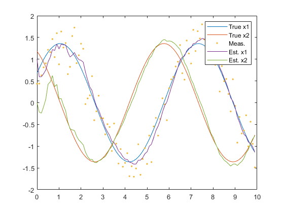
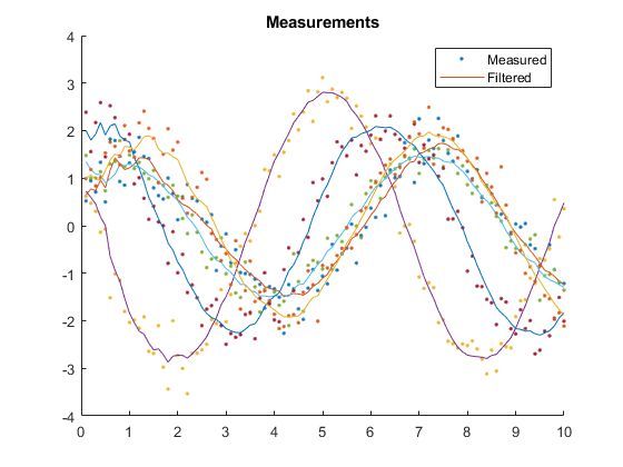
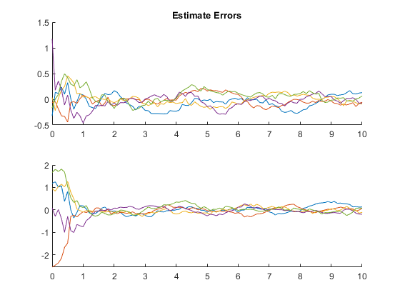
Example of Monte-Carlo Testing
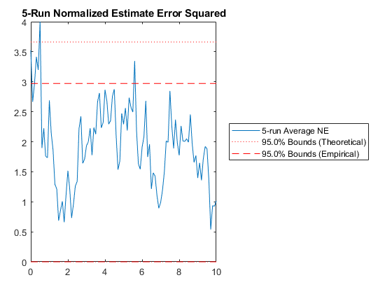
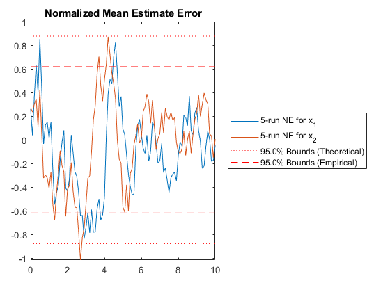
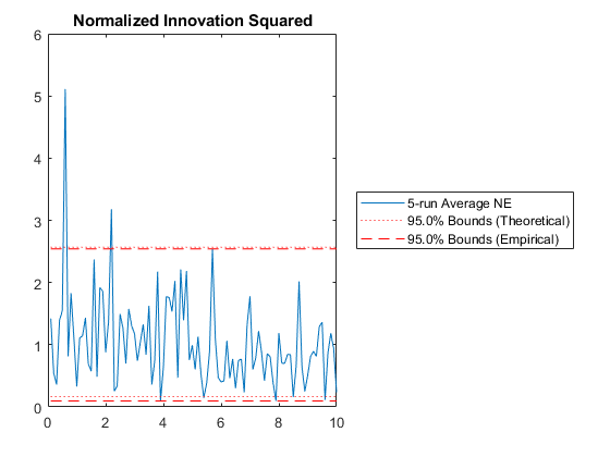
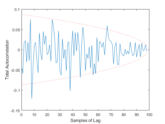
We can run multiple Monte-Carlo simulations automatically using the framework.
% Simulate the same thing as above, but do it 5 times with different
% random draws, and then show statistics.
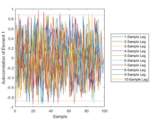
kffmct(5, [0 10], dt, x_hat(:, 1), P_0, options);NEES: Percent of data in theoretical 95.0% bounds: 99.0%
NMEE: Percent of data in theoretical 95.0% bounds: 99.5%
NIS: Percent of data in theoretical 95.0% bounds: 93.0%
TAC: Percent of data in theoretical 95.0% bounds: 93.9%
AC: Percent of data in theoretical 95.0% bounds: 97.8%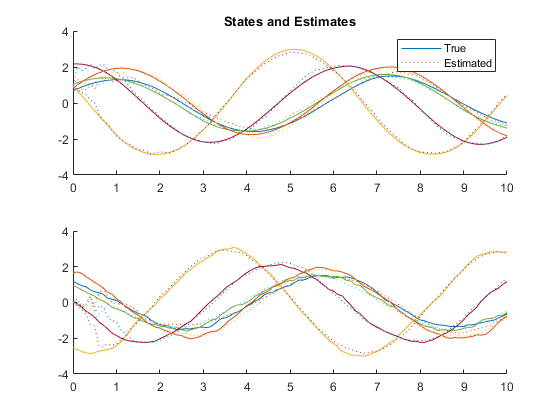
See Also
*kf v1.0.3 February 4th, 2023
©2023 An Uncommon Lab