by An Uncommon Lab

mndpdf

This function computes the probability density of a zero-mean multivariate normal distribution with the given covariance, X, at the specified values, x.

 p = mndpdf(x, X);

Inputs

Outputs

Example

Let's start with the most basic case: a 1-dimensional unit normal distribution with zero mean. At x = 1, we expect the theory that the PDF will be about 0.242.

x = 1;
X = 1;
mndpdf(x, X)

ans =
    0.2420

Example: 2-Dimensional Covariance Matrix

Let's try a multivariate distribution:

x       = [1; 0]
sigma_1 = 1;
sigma_2 = 2;
X       = diag([sigma_1^2, sigma_2^2])
mndpdf(x, X)

x =
     1
     0
X =
     1     0
     0     4
ans =
    0.0483

Is that correct? Well, since the two variables are independent (the covariance matrix is diagonal), then the PDF is just the PDF of the first value taken independently times the PDF of the second value taken independently, like so:

mndpdf(x(1), sigma_1^2) * mndpdf(x(2), sigma_2^2)

ans =
    0.0483

Example: Plot and Histogram

Let's look at the PDF of a random 2D covariance matrix.

dx         = 0.1;
[x1m, x2m] = meshgrid(-10:dx:10);  % Make a point for each dx of x1 and x2.
x          = [x1m(:).'; x2m(:).']; % Make vectors.
X          = [2 1; 1 4];           % An arbitrary covariance matrix
p          = mndpdf(x, X);
pm         = reshape(p, size(x1m));
surf(x1m, x2m, pm, 'EdgeColor', 'None')
xlabel('x_1');
ylabel('x_2');
zlabel('Probability Density');
title(colorbar(), 'PD')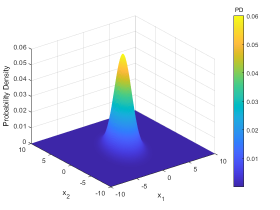

Let's draw a bunch of random samples from our covariance matrix and look at the histogram. It should line up nicely.

draws = mnddraw(X, 10000);
histogram2(draws(1,:), draws(2,:), 'Normalization', 'PDF');
hold on;
surf(x1m, x2m, pm, 'EdgeColor', 'None')
hold off;
xlabel('x_1');
ylabel('x_2');
zlabel('Probability Density');
title(colorbar(), 'PD')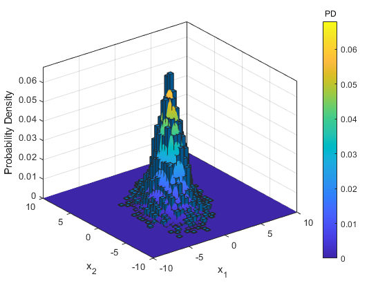

If we very roughly "integrate" the PDF over the space, the result should be 1:

sum(mndpdf(x, X) * dx^2)

ans =
    1.0000

Example: Error Conditions

What happens if we use an invalid covariance matrix, where the PDF cannot be evaluated?

[p, err] = mndpdf([1; 2], [0 0; 0 1])

p =
     0
err =
  logical
   1

It doesn't throw an error, but instead returns 0 with an error flag.