ukf

Run one update of a basic unscented (sigma point) Kalman filter. The advantage of a UKF over a traditional extended Kalman filter is that the UKF can be more accurate when the propagation/measurement functions are not zero-mean wrt the error (that is, they are significantly nonlinear in terms of their errors). Further, since a UKF doesn't require Jacobians, it's often easier to use a UKF than an EKF. The disadvantage is increased runtime. Though a UKF operates "on the order" of an EKF, in implementation it often takes several times longer.

[x_k, P_k, P_xc_k] = ukf( ...
    t_km1, t_k, x_km1, P_km1, u_km1, z_k, ...
    f, h, Q_km1, R_k, ...
    alpha, beta, kappa, ...
    P_cc, P_xc_km1, ...
    (etc.))

Inputs

t_km1	Time at sample k-1
t_k	Time at sample k
x_km1	State estimate at sample k-1
P_km1	Estimate covariance at sample k-1
u_km1	Input vector at sample k-1
z_k	Measurement at sample k
f	Propagation function with interface: `x_k = f(t_km1, t_k, x_km1, u_km1, q_km1)` where `q_km1` is the process noise at sample k-1
h	Measurement function with interface: `z_k = h(t_k, x_k, u_km1, r_k)` where `r_k` is the measurement noise at sample k
Q_km1	Pocess noise covariance at sample k-1
R_k	Measurement noise covariance at sample k
alpha	Optional tuning parameter, often 0.001
beta	Optional tuning parameter, with 2 being optimal for Gaussian estimation error
kappa	Optional tuning parameter, often 3 - `nx`, where `nx` is the dimension of the state
P_cc	Optional consider covariance (presumed constant)
P_xc	Optional state-consider covariance at k-1
(etc.)	Additional arguments to be passed to `f` and `h` after their normal arguments

Outputs

x	Upated estimate at sample k
P	Updated estimate covariance at sample k
P_xc	When using consider covariance (P_cc and P_xc), this is the updated covariance between the state and consider parameters at sample k.

Example

We can quickly create a simulation for discrete, dynamic system, generate noisy measurements of the system over time, and pass these to an unscented Kalman filter.

First, define the discrete system.

rng(1);
dt    = 0.1;                                  % Time step
F_km1 = expm([0 1; -1 0]*dt);                 % State transition matrix
G_km1 = [0.5*dt^2; dt];                       % Process-noise-to-state map
Q_km1 = G_km1 * 0.5^2 * G_km1.';              % Process noise variance
R_k   = 0.1;                                  % Meas. noise covariance

Make propagation and observation functions. These are just linear for this example, but ukf is meant for nonlinear functions.

f = @(t0, tf, x, u, q) F_km1 * x + q;
h = @(t, x, u, r) x(1) + r;

Now, we'll define the simulation's time step and initial conditions. Note that we define the initial estimate and set the truth as a small error from the estimate (using the covariance).

n       = 100;                     % Number of samples to simulate
x_hat_0 = [1; 0];                  % Initial estimate
P       = diag([0.5 1].^2);        % Initial estimate covariance
x_0     = x_hat_0 + mnddraw(P, 1); % Initial true state

Now we'll just write a loop for the discrete simulation.

% Storage for time histories
x     = [x_0, zeros(2, n-1)];                         % True state
x_hat = [x_hat_0, zeros(2, n-1)];                     % Estimate
z     = [x_0(1) + mnddraw(R_k, 1), zeros(1, n-1)];    % Measurement
 
% Simulate each sample over time.
for k = 2:n
 
    % Propagate the true state.
    x(:, k) = F_km1 * x(:, k-1) + mnddraw(Q_km1, 1);
    
    % Create the real measurement at sample k.
    z(:, k) = x(1, k) + mnddraw(R_k, 1);
 
    % Run the Kalman correction.
    [x_hat(:,k), P] = ukf((k-1)*dt, k*dt, x_hat(:,k-1), P, [], z(:,k), ...
                          f, h, Q_km1, R_k);
 
end

Plot the results.

figure(1);
clf();
t = 0:dt:(n-1)*dt;
plot(t, x, ...
     t, z, '.', ...
     t, x_hat, '--');
legend('True x1', 'True x2', 'Meas.', 'Est. x1', 'Est. x2');
xlabel('Time');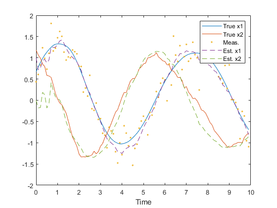

Note how similar this example is to the example of lkf.

Reference

Wan, Eric A. and Rudoph van der Merwe. "The Unscented Kalman Filter." Kalman Filtering and Neural Networks. Ed. Simon Haykin. New York: John Wiley & Sons, Inc., 2001. Print. Pages 221-276.

Docs

ukf

Inputs

Outputs

Example

Reference

See Also

Table of Contents