Intro
Let's suppose you've agreed to a rather odd travel program, where you're going to be suddenly transported to a randomly selected country, and your job is to figure out where you end up. So, here you are in some new country, and all countries are equally likely. You make a list of places and probabilities that you're in those places (all equally likely at about 1/200 for 200 countries).
| Place | Probability |
|---|---|
| Afghanistan | 0.005 |
| Albania | 0.005 |
| … | |
| Mauritius | 0.005 |
| Mexico | 0.005 |
| … | |
| Zambia | 0.005 |
| Zimbabwe | 0.005 |
You look around and appear to be in a restaurant. Some countries have more restaurants (per capita/per land area) than others, so you decrease the odds that you're in Algeria or Sudan and increase the odds that you're in Singapore or other high-restaurant-density places.
| Place | Prior Prob. | Prob. of Restaurant, given Country | Result |
|---|---|---|---|
| … | |||
| Algeria | 0.005 | 0.01 | 0.00005 |
| … | |||
| Singapore | 0.005 | 0.3 | 0.0015 |
| … | |||
| … | |||
| Sudan | 0.005 | 0.01 | 0.00005 |
| … |
That is, you just multiply the probability that you were in a country with the probability of finding oneself in a restaurant in that country, given that one were already in the country, to obtain the new probability. (The last column isn't actually a probability until it's scaled so that it sums to 1, but only the relative values matter, so it's a probability as far as anyone cares.)
After a few moments, the waitress brings you sushi, so you decrease the odds for Tajikistan and Paraguay and correspondingly increase the odds on Japan, Taiwan, and such places where sushi restaurants are relatively common.
| Place | Prior Prob. | Prob. of Sushi given Restaurant, Country | Result |
|---|---|---|---|
| … | |||
| Japan | 0.0015 | 0.3 | 0.00045 |
| … | |||
| Tajikistan | 0.0005 | 0.005 | 0.0000025 |
| … |
You pick up the chopsticks and try the sushi, discovering that it's excellent. Japan is now by far the most likely place, and though it's still possible that you're in the United States, it's not nearly as likely (sadly for the US).
| Place | Prior Prob. | Prob. of Good Sushi | Result |
|---|---|---|---|
| … | |||
| Japan | 0.00045 | 0.75 | 0.0003375 |
| … | |||
| United States | 0.00005 | 0.1 | 0.000005 |
| … |
Those “probabilities” are getting really hard to read with all those zeros in front. All that matters is the relatively likelihood, so perhaps you scale that last column by the sum of the whole column. Now it's a probability again, and it looks something like this:
| Place | Probability |
|---|---|
| … | |
| Japan | 0.7 |
| … | |
| United States | 0.01 |
| … | |
| Taiwan | 0.1 |
| … |
Now that you're pretty sure it's Japan, you make a new list of places inside Japan to see if you can continue to narrow it down. You write out Fukuoka, Osaka, Nagoya, Hamamatsu, Tokyo, Sendai, Sapporo, etc., all equally likely (and maybe keep Taiwan too, just in case).
| Place | Probability |
|---|---|
| … | |
| Fukuoka | 1/44 |
| … | |
| Hamamatsu | 1/44 |
| … | |
| Osaka | 1/44 |
| … | |
| Taiwan | 1/44 |
| … |
Now the waitress brings unagi. You can get unagi anywhere, but it's much more common in Hamamatsu, so you increase the odds on Hamamatsu and slightly decrease the odds everywhere else.
| Place | Prior Prob. | Prob. of Unagi | Result |
|---|---|---|---|
| … | |||
| Fukuoka | 1/44 | 0.1 | 0.0022 |
| … | |||
| Hamamatsu | 1/44 | 0.3 | 0.0068 |
| … | |||
| Osaka | 1/44 | 0.1 | 0.0022 |
| … | |||
| Taiwan | 1/44 | 0.05 | 0.0011 |
| … |
By continuing in this manner, you may eventually be able to find that you're eating at a delicious restaurant in Hamamatsu Station — a rather lucky random draw.
There's nothing especially odd about the process you've gone through (except that you had such good restaurant data), and everyone would agree that it was pretty reasonable. It was also basically a particle filter, a method for determining unknown things, like location, from measurements of other things, like cuisine, using different probabilities about what you'd observe under different hypotheses. In fact, it's sort of like an automated application of the scientific method, isn't it?
When performed as part of an algorithm, this type of thing is called recursive state estimation. Unfortunately, only a small fraction of mechanical engineers, electrical engineers, and data scientists receive any formal education on the subject, and even fewer develop an intuitive understanding for the process or have any knowledge about practical implementation. While there are very many good books on the math behind it and the details of how to apply it to certain specific problems, this article will take a different approach. We’ll focus on developing:
- an intuition for recursive state estimation,
- a broad knowledge of the strongest and most general types,
- and a good idea of the implementation details.
Once one has a good foundation for these things, it becomes much easier to look up specific algorithms in the filter literature, customize them, adapt them to code, correct problems, and explain performance to others.
Interestingly, the most intuitive forms of recursive estimation are only recently becoming popular, so we’re going to look at their history entirely backwards: starting from the most recent types, like particle filters, and working back into the ancient past (the 1960s) for the breakthrough that enabled the Apollo navigation algorithms to keep a spacecraft on a course to the moon: the Kalman filter.
The target audience is engineers, scientists, makers, and programmers who need to design a system to understand a process, along with the systems engineers and team leads who need a better understanding of what their teams are building. To approach the topic, we'll begin by creating a rough sketch of filter ideas. Then, we'll fill in the sketch with more and more detail. The first part might take a couple of hours, and the second part will take about half that, depending on how deeply one chooses to read. Then there are some appendices for extra implementation notes and exercise with these topics. Anyone can follow the basic ideas here, but a little probability theory and basic linear algebra will help to follow the math and the reference material as we get more detailed. We’ll point out several good resources along the way. With that, let’s get started.
The Particle Filter
Particle filters can be pretty easy, and there are about as many forms as there are problems to solve. We'll look at a simple type of particle filter called a bootstrap filter to build an understanding of the basics.
One Iteration of a Particle Filter
Particles filters work like this: First, we ask, “What things could be happening, and how likely is each thing?” Then, “For each thing that could be happening, what would I expect to observe?” Then, “How likely is each thing, given what I've now actually observed?” We then repeat.
For example, suppose we approximately know the original position of a bouncing ball, but don't know much about the velocity. Let's create a bunch of “hypothesis” balls, randomly dispersed around where we think the real ball is and with random velocities. And let's say that, as far as we know, these are all equally likely candidates for the true ball's position and velocity (its state).
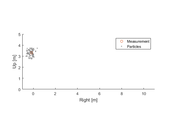
This list of hypothetical balls is like the list of countries.
Each hypothetical ball's state is called a particle, and the likelihood that the particle best represents the true state is the particle weight. So, for each particle, we have a hypothetical ball's position and velocity, as well as a measure of the likelihood, from 0 to 1, that the ball describes the truth, where 1 is complete certainty and 0 represents no possibility at all. E.g., the particle weight for South Georgia Island goes to exactly 0 given that there are no sushi restaurants on South Georgia Island (despite all of the fish that are consumed there).
Now, a moment later, we get a measurement of the ball's position.
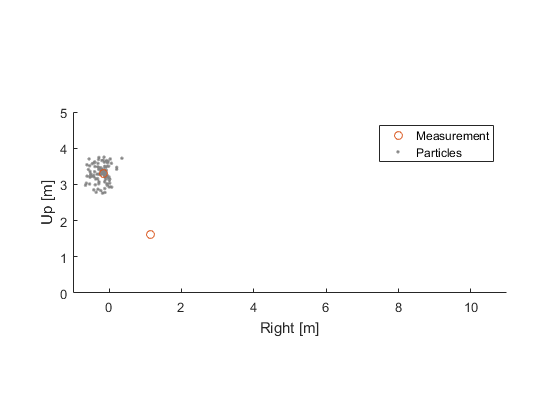
How did the ball arrive at this position? Did it go up and slowly arc back down? Did it go down, bounce off the floor, and come back up? We don't know yet. Either path is equally likely.
We also know that the measurement isn't perfect; it has some noise. So, let's take each hypothesis, propagate it forward to the time of the measurement, and see how well it predicts the real measurement. Let's call \(\hat{x}_{i, k-1}\) the state (the two position terms and the velocity terms) of the \(i\)th particle at the last sample time, and let's call \(\hat{x}_{i,k}\) the state at the current sample time. We use hats to denote estimates and \(k\) for the sample. We know how bouncing balls work, so we can propagate from the previous time to the current time using a propagation function, \(f\).
$$ \hat{x}_{i,k} = f(\hat{x}_{i,k-1}) $$This updates the position and velocity for each of the \(n\) particles by starting with the previous position and velocity and calculating the parabola the ball makes due to gravity, when/if it intersects the floor, and the trajectory from the floor back upwards, etc., until it reaches the current time. The propagation function is therefore a tiny simulation.
Given the updated position, we predict what we'd expect to measure for each particle, using a known observation function, \(h\).
$$ \hat{z}_{i,k} = h(\hat{x}_{i,k}) $$where the hat denotes a predicted measurement, to help us distinguish it from the real measurement, \(z_k\). For our problem, the observation function simply returns the position of the ball.
Some particles predict the measurement quite well, and others do poorly.
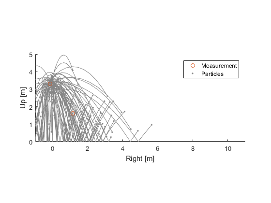
We can take the difference between each ball's new position and the measurement (\(z_k - \hat{z}_{i,k}\)) and say, “What are the odds of seeing a measurement error this big, given what we know about how noisy the measurements can be?” The really bad predictions have low odds, whereas the good predictions will have high odds.
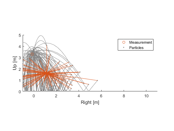
So, we have a probability for the measurement error for each hypothetical ball. We can multiply each particle's weight by this probability. The result is that particles that best predict the measurement end up with the highest weight. Let's show that by shading the trajectories according to their new weights:
(Note that, after doing this multiply, the sum of the weights won't be 1. We can renormalize by dividing all of the weights by the sum of all of the weights.)
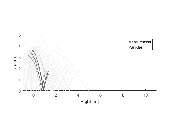
Using these weights, we can calculate the weighted average of all of the hypothetical balls. This might provide the best estimate of the state (there are also many other ways we could use the probabilities to calculate a best estimate, with the weighted average being the most simplistic).
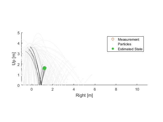
At this point, we have an updated state estimate and associated uncertainty, here represented as a finite collection of particles. We could now wait for another measurement to come in and run through this process once more. We'd propagate each ball to the time of the measurement, calculate the probability of the error between the measurement and the propagated ball, and update that ball's probability. So, let's go through one more cycle.
Another Iteration, Adding in Resampling and Regularization
Propagate.
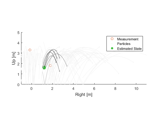
Some particles predict the new measurement well, and some no longer predict well. Update the probability of each.
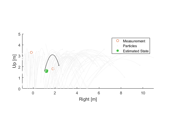
Notice that some of our original hypothetical balls are useless now. There's just no way they represent the truth. Plus, they're all starting to spread out pretty far. Eventually, they'll all be too far away from the truth, and our filter will fall apart. The key that makes the particle filter work is that the set of particles is recalculated every once in a while (or even after each update), just like when we switched from a list of potential worldwide locations to a finer list of locations in Japan. There are a lot of ways to do this, but here's an easy one:
- Create a new set of particles by randomly choosing particles from the current set according to the particle weight. So, in general, particles with a weight of 0.04 will be drawn twice as often as particles with a weight of 0.02.
- Once the new set of particles is created, set all of the weights back to 1/N. The dispersion of the uncertainty is now represented in the presence of different particles, and not by the particle weights. Just to be clear: there will be many duplicated particles at this point.
- Calculate the sample covariance of the new set of particles, or some other measure of their dispersion. The sample covariance is particularly easy: $$ P_k = \frac{1}{n-1} \sum_i^n (\hat{x}_{i,k} - \bar{x}) (\hat{x}_{i,k} - \bar{x})^T $$ where \(\bar{x}\) is the average of all particles and \(^T\) means “transpose”.
- Make a bunch of Gaussian random draws from the sample covariance matrix (see the appendix). Multiply these draws by some small tuning parameter, giving a set of perturbations. Add a perturbation to each particle.
This creates a set of new particles scattered around the high-probability areas of the state space. The first two steps are called resampling, and the final two are called regularizing the particles. Let's do that for the current set of particles:
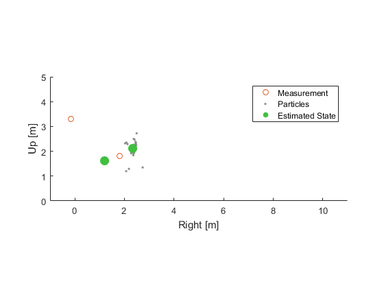
Outline of a Bootstrap Filter
We can now continue with the next measurement, and then the next, and the next, keeping with the process we've set up:
- Propagate the particles.
- Determine how likely each particle is given the new measurement.
- Update their weights (and renormalize so that the sum of all of the weights comes to 1).
- Calculate the state estimate, e.g. with a weighted average.
- If resampling the particles this time, randomly select particles according to their weights, and then return the weights to 1/N.
- If regularizing the particles this time, perturb the new set of particles with small random draws.
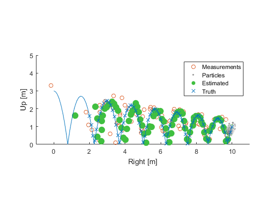
Going back to the ball example, here's the result converging over time, with the uncertainty clearly clustering around the true state (blue):
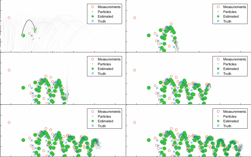
After ten seconds:
Assumptions, Advantages, and Disadvantages
What's required for all of this to work? Just a couple of simple things:
- You can approximately describe how the states change over time.
- You can approximately determine the likelihood of a hypothetical measurement error.
The advantages of particle filtering are pretty clear: you can coarsely estimate a state with very little theoretical work and for many different types of problems. The uncertainty (set of particles) can even be spread across multiple regions of the state space, representing a multimodal probability distribution. Further, the particle filtering process is easily customizable to different problems (e.g., when and how to resample, how to evaluate the measurement error, how to position particles in the first place). This makes particle filtering flexible and broadly useful.
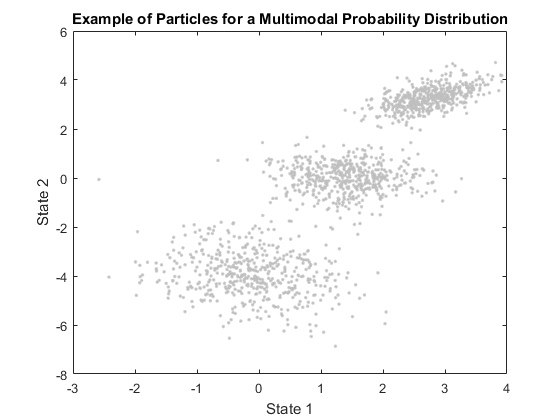
The disadvantages are also pretty clear:
- Particle filters generally require a large number of particles, which can take substantial runtime. It's not uncommon for even the simplest particle filter to use 1000 particles, which requires 1000 simulations per measurement. The necessary number of particles becomes enormous as the dimension of the state grows. (Our problem would have benefitted substantially from 1000 particles, but it would have been harder to understand the plots with such a large number of particles.)
- Representing the uncertainty as a set of particles and weights — a discrete probability distribution — means that the best estimate of the state is usually pretty coarse, and so particle filters work poorly for problems that require high accuracy.
- When better performance is required, particle filters must often be tailored significantly to fit each individual state estimation problem, and this can take a long time, not least because testing requires one to run the filter, which can itself take a long time. For the same reason, it's hard to find a useful general-purpose particle filter, though the bootstrap filter is fine for simple problems.
Particle filters are only gaining popularity relatively recently, owing to the fact that processing power and distributed computing is now so cheap and easy to wield. Further, there are many new techniques for particle filters that can reduce runtime and increase accuracy. However, for applications that need speed, we generally need a different filtering architecture.
The Sigma-Point Filter
Uncertainty as a Covariance Matrix
In sigma-point filters (also called unscented filters), we don't represent uncertainty with a big bunch of scattered particles, but instead we assume that the uncertainty has a Gaussian (normal) distribution and is centered on the current best estimate:
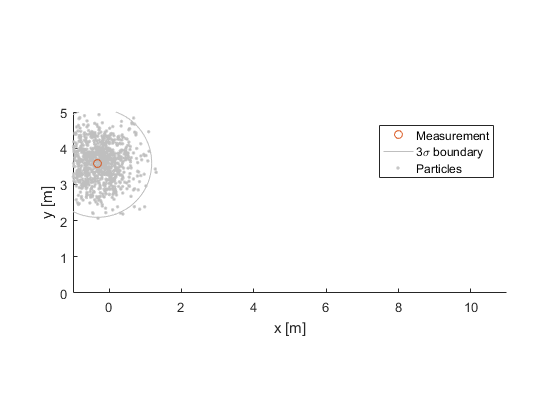
We can therefore represent the uncertainty with a covariance matrix, like we calculated for the particles, above. We're visualizing the covariance as an ellipse around the state estimate, where the ellipse is drawn at the 3σ boundary (the true state is therefore inside this ellipse about 99.7% of the time). The 1000 particles are drawn only for the sake of comparison.
Propagation
When a new measurement comes in, we'll need to propagate this uncertainty forward to the time of the measurement. How do we do that? Sigma-point filters do this by first placing a few sigma points around the current estimate.
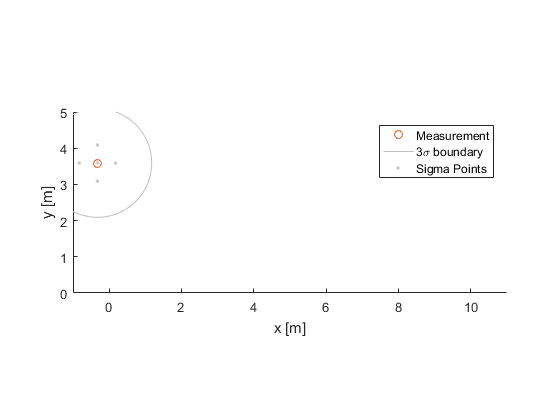
Sigma points are the same as particles, but we are particular about where we place them, and we don't need to keep track of individual weights. The sigma points will sit on the principal axes of the uncertainty ellipsoid around the current estimate (usually, a much smaller ellipse than the one we've drawn). Note that we're only looking at two dimensions of the problem; there are sigma points in the two velocity dimensions too, as well as in the noise dimensions, which we'll get to more below.
The estimate from the last sample, \(\hat{x}^+_{0,k-1}\), and each sigma point, \(\hat{x}^+_{i,k-1}\), are then propagated forward to the time of the new measurement.

(The plus sign denotes that the estimate was corrected with the measurements available at the time; we'll cover this more below.)
Just like for particle filters, the sigma points tend to spread out (uncertainty usually grows) during propagation. And, just like for particle filters, we can calculate a new state estimate as a weighted average of the sigma points.
Similar to before, the propagation function is:
$$ \hat{x}^-_{i,k} = f(\hat{x}^+_{i,k-1}, q_{i,k-1}) $$but there's something new here: we've added \(q_{i,k-1}\), which represents process noise — unknowns that affect the propagation, like perhaps a random acceleration due to changes in the wind. What value would we use for it? Just like we have sigma points spread around in state space, so too we have sigma points spread around in process noise space. So, if there are 3 separate things that randomly affect the propagation, then \(q_{i,k-1}\) is a 3 dimensional vector. In sigma-point filters, it's assumed that the process noise is Gaussian, so the uncertainty is specified as a covariance matrix, \(Q\). Even when it's not Gaussian, this is usually a good approximation for any unimodal distribution. So, the sigma points in process-noise-space are just like sigma points in state-space, and taken together are just the big set of sigma points.
Once we've calculated the sigma points and propagated each, we calculate the mean predicted state as a weighted average:
$$ \hat{x}^-_k = W_0 \hat{x}^-_{0,k} + W \sum_{i=1}^n \hat{x}^-_{i,k} $$where \(\hat{x}^-_{0,k}\) is the “middle” sigma point. All sigma points use the same weight, \(W\), except for the middle point, which usually uses a larger \(W_0\) because we trust it more. We now have the best prediction of the state at sample \(k\), and we marked it with a minus sign to denote “before correction” with the new measurement, or a priori.
We can then calculate the sample covariance around this new estimate, giving the covariance of the predicted state (again, the middle point has a larger weight, \(W_c\), than the others, but the idea is the same).
$$ P^-_k = W_c (\hat{x}^-_{0,k} - \hat{x}^-_k) (\hat{x}^-_{0,k} - \hat{x}^-_k)^T + W \sum_{i=1}^n (\hat{x}^-_{i,k} - \hat{x}^-_k) (\hat{x}^-_{i,k} - \hat{x}^-_k)^T $$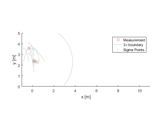
We now have an idea of what the state is when the measurement comes in, as well as the uncertainty associated with our prediction.
Correcting the Estimate
Now of course, we need to use the measurement information to somehow correct the state estimate and covariance. Just like we have a predicted state for each sigma point, \(\hat{x}^-_{i,k}\), and the overall predicted state, \(\hat{x}^-_k\), we make an overall predicted measurement, \(\hat{z}_k\) by making a prediction for each sigma point:
$$ \hat{z}_{i,k} = h(\hat{x}^-_{i,k}, r_{i,k}) $$(where \(r_{i,k}\) is the measurement noise with covariance \(R\), which is analogous to the process noise) and then calculating the weighted mean:
$$ \hat{z}_k = W_0 \hat{z}_{0,k} + W \sum_{i=1}^n \hat{z}_{i,k} $$We'll use this predicted measurement to correct the predicted state like so:
$$y_k = z_k - \hat{z}_k$$ $$\hat{x}^+_k = \hat{x}^-_k + K y_k$$where the plus sign denotes “after measurement correction” or a posteriori. For historical reasons, \(y_k\) is called the innovation vector, measurement prediction error, or residual. It's a vector pointing from our predicted measurement to the actual measurement, and \(K\) determines how a vector in measurement space maps to a correction in state space.
Let's think of some desirable properties for \(K\). If our knowledge of the state were really good already, and the measurements were so noisy that they weren't that useful, then \(K\) should be small — we probably don't want much correction to the prediction. For example, if someone cries, “Wolf!”, but that guy is always crying wolf, and nobody's seen a wolf around here for ages, then you ignore him, or at least mostly ignore him.
On the other hand, if our knowledge of the state were pretty bad, and the measurements were known to be pretty good (wolves are often seen around here, and the guy who cried wolf is usually right about these types of things), then we'd want to trust the measurements a lot more. In that case, we'd want \(K\) to be big (we might not have predicted that there's a wolf, but there certainly seems to be one now).
Turning this into math, we represent the relationship between the uncertainty in the state (is there a wolf?) and the measurement error (someone cries wolf erroneously) with a covariance matrix, \(P_{xy}\). We represent the uncertainty of the measurement error (someone cries wolf erroneously) with another covariance matrix, \(P_{yy}\). If we're really sure that there is or isn't a wolf, \(P_{xy}\) will be quite small. If there are no pranksters around, \(P_{yy}\) will be small too, but no smaller than our fundamental uncertainty in whether there's a wolf around or not. If there are pranksters about, then \(P_{yy}\) will be large — lots of error.
We calculate these as weighted sample covariances, similar to what we did for the particle filter.
$$ P_{xy} = W_c (\hat{x}^-_{0,k} - \hat{x}^-_k) (\hat{z}_{0,k} - \hat{z}^-_k)^T + W \sum_{i=1}^n (\hat{x}^-_{i,k} - \hat{x}^-_k) (\hat{z}_{i,k} - \hat{z}^-_k)^T $$ $$ P_{yy} = W_c (\hat{z}_{0,k} - \hat{z}^-_k) (\hat{z}_{0,k} - \hat{z}^-_k)^T + W \sum_{i=1}^n (\hat{z}_{i,k} - \hat{z}^-_k) (\hat{z}_{i,k} - \hat{z}^-_k)^T $$Switching back to the bouncing ball, our measurement is the ball's position, so we can draw both \(P_{xy}\) and \(P_{yy}\) for the position error in the same plot:
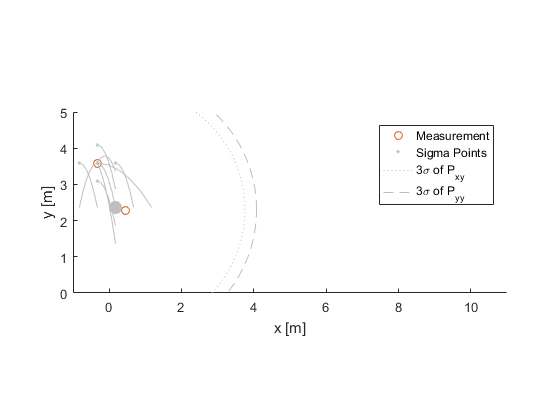
Using these covariance matrices, let's try a simple ratio: the uncertainty in our prediction (\(\hat{x}^-_k\) and \(\hat{z}_k\)) “over” the uncertainty in our predicted measurement error (\(y_k = z_k - \hat{z}_k\)), in a matrix sense:
$$ K = P_{xy} P_{yy}^{-1} $$It turns out that this “ratio” is a really good choice. For linear systems, it will produce the estimate with the least squared error in general. It's called the Kalman gain.
Note how, in our case, the ellipsoids for \(P_{xy}\) and \(P_{yy}\) are pretty close together. This means we have a lot of uncertainty about where the ball will go, and we have a little bit more uncertainty about what we'll measure. Since the Kalman gain is like a ratio, and our “numerator” and “denominator” terms are pretty close together, our gain will be close to the identity matrix for the position part of the state. A corresponding factor will update the velocity part of the state. The actual Kalman gain for this example is:
$$ K = \begin{bmatrix} 0.8 & 0 \\ 0 & 0.8 \\ 1.2 & 0 \\ 0 & 1.2 \end{bmatrix} $$where the two position terms are the top part of the state, and the two velocity terms are on bottom. This says that the update will be most of the difference (0.8) from the predicted position to the measured position, and correspondingly, velocity will be increased in the same direction (1.2).
We now have the final state estimate for the current measurement:
$$ \hat{x}^+_k = \hat{x}^-_k + K y_k $$Correcting the Covariance
We're not done quite yet. The correction also affects the uncertainty in our new estimate, and we haven't updated the sigma points, so we haven't represented how the correction reduces our uncertainty. We can account for this by correcting the sigma points too, in the same way we corrected the state.
$$ \hat{x}^+_{i,k} = \hat{x}^-_{i,k} + K \left( z_k - \hat{z}_{i,k} \right) $$Then, we can calculate the new covariance matrix as a sample covariance of the corrected sigma points, \(P^+_k\).
$$ P^+_k = W_c (\hat{x}^+_{0,k} - \hat{x}^+_k) (\hat{x}^+_{0,k} - \hat{x}^+_k)^T + W \sum_{i=1}^n (\hat{x}^+_{i,k} - \hat{x}^+_k) (\hat{x}^+_{i,k} - \hat{x}^+_k)^T $$However, there's no need to literally correct every sigma point, because the definition for the Kalman gain results in a faster way:
$$ P^+_k = P^-_k - K R_k K^T $$where \(R_k\) is the covariance of the measurement error, such as we might have from the specification sheet for our position sensors. We don't work out the proof here, but we can interpret the result pretty well: the Kalman gain determines how much of the measurement noise we can subtract from the propagated covariance matrix. Recall that, if the measurement noise were large, then \(K\) would be small (measurement noise is in the “denominator”), and thus very little of the measurement noise would be subtracted off. If the measurement noise were small, then \(K\) would be larger, and we'd subtract a larger part of the (smaller) measurement noise. The result is that the right amount of \(R\) is removed over time.
That means large Kalman gains subtract more, leaving a small covariance matrix, which reflects more certainty in the estimate.
Here are the results. Notice how the 3σ boundary is smaller than for our starting estimate.
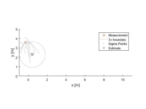
That completes one cycle of the sigma-point filter! When a new measurement comes in, we can do it all over again. Going forward 10 seconds, here are the results:
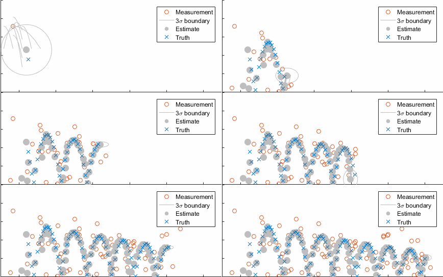
Look at how the uncertainty in the up-down element gets really small at the top of the bounce, because we know the ball will slow down there, whereas the uncertainty in the left-right element is pretty well constant by the end, since the rightward velocity doesn't change.
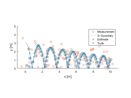
By the end, the estimate is well-aligned with the truth, despite the really terrible measurements. In fact, the measurements for this example were actually allowed to be worse than those used for the particle filter, and yet the accuracy is clearly far better, owing to the fact that particles create a coarse representation of the distribution, whereas sigma-point filters are nice and smooth.
Outline of a Sigma-Point Filter
- Set up the initial sigma points from the last state estimate and covariance matrix. We'll need a positive and negative sigma point for each dimension of the state, for each dimension of the process noise, and for each dimension of the measurement noise, plus 1 more for the middle sigma point.
- Propagate each of the sigma points forward to the time of the new measurement.
- Create the predicted measurement for each sigma point, including sensor noise.
- Use a weighted sum of the sigma points as the mean predicted state and mean predicted measurement.
- Calculate the sample covariance between the propagated sigma points about the mean state and the predicted measurements about the mean predicted measurement, \(P_{xy}\).
- Calculate the sample covariance of the measurement errors about the mean measurement, \(P_{yy}\).
- Calculate the Kalman gain, \(K\).
- Correct the state estimate and covariance matrix.
Assumptions, Advantages, and Disadvantages
When the various sources of uncertainty (previous uncertainty, process noise, and measurement noise) are unimodal and uncorrelated, sigma-point filters are a powerful option. Some advantages:
- Within their assumptions, they are generally more accurate than particle filters, since they don't rely on random particles.
- They're far, far faster than particle filters. Where a particle filter may need 1000 points, a sigma-point filter may need only 9 or so.
- Their assumptions apply to many different realistic problems, and setting up a sigma-point filter requires only defining the propagation function, measurement function, process noise covariance, and measurement noise covariance, all of which are necessary for particle filters too.
- There are standard forms for sigma-point filters, so it's relatively easy to find a good reference in a book or journal.
We could list a few disadvantages though.
- Odd problems can result in a sigma-point filter “falling apart”. For instance, in our ball problem, if the time step were larger, the sigma points would become very “confused” across one or two bounces, and may result in sample covariance matrices that make no sense. It can be difficult to avoid this, whereas particle filters wouldn't have this problem.
- While they're much faster than particle filters, they are also much slower than extended Kalman filters, which we'll get to in a moment.
Interlude: Expectation and Covariance
Before we move on to the next filter, let's take a moment to review some probability theory that will help out. First is the expectation operator. If \(a\) is some random number, its expected value, \(E(a)\), is its mean, which we might call \(\bar{a}\) for brevity. So, if \(a\) represents rolls of a 6-sided die, then the expected value is 3.5, despite that we can't actually roll a 3.5.
The second important idea is covariance. We looked at sample covariance above, where we used a bunch of points to calculate a covariance, but now we'll talk about the idea of covariance. The covariance of \(a\), let's say \(P_{aa}\), is:
$$ P_{aa} = E( (a - E(a)) (a - E(a))^T ) $$When \(a\) is a scalar, there's no “co-” in there; it's just called variance:
$$ P_{aa} = E((a - \bar{a})^2) $$If we call \(a - \bar{a}\) the error or residual, then the above tells us that the variance is simply the mean squared error of \(a\) about its mean. Further, the standard deviation is the square root of the variance:
$$ \sigma_a = \sqrt{P_{aa}} $$and so the standard deviation is also the square root of the mean squared error, sometimes called root-mean-square (RMS) error.
If \(b\) represents rolls from a totally different die, and we're rolling \(a\) and \(b\) together, then what's the covariance between \(a\) and \(b\), \(P_{ab} = E( (a - \bar{a}) (b - \bar{b})^T )\)? Sometimes \(a - 3.5\) would be positive and sometimes negative, and likewise for \(b - 3.5\). Their product would be sometimes positive and sometimes negative, and averaging a bunch of these would come to 0, because the rolls are uncorrelated. That is, if \(a\) and \(b\) are uncorrelated, their covariance is 0.
Nothing much is different when we upgrade from a random number to a random vector. Let's consider a two-element vector \(c = \begin{bmatrix} a & b \end{bmatrix}^T\), where \(a\) and \(b\) are the same dice rolls as above.
$$ \begin{align} P_{cc} & = E( (c - E(c)) (c - E(c))^T) \\ & = \begin{bmatrix} E((a-\bar{a})^2) & E((a-\bar{a})(b-\bar{b})) \\ E((b-\bar{b})(a-\bar{a})) & E((b-\bar{b})^2) \end{bmatrix} \\ & = \begin{bmatrix} P_{aa} & 0 \\ 0 & P_{bb} \\ \end{bmatrix} \\ & \\ \end{align} $$When the elements of \(c\) are correlated, some of those off-diagonal terms will be non-zero. For instance, let's reassign \(b\) so that \(b = 2 a + 1\).
$$ \bar{b} \equiv E(b) = E( 2 a + 1 ) $$We can move the factor of 2 and the added 1 outside of the expectation:
$$ \bar{b} = 2 E(a) + 1 = 2 \bar{a} + 1 $$Now for the variance part:
$$ b - \bar{b} = 2 a + 1 - 2 \bar{a} - 1 = 2 (a - \bar{a}) $$The variance of \(b\) is now:
$$ P_{bb} = E( (b - \bar{b}) (b - \bar{b}) ) = 4 E((a - \bar{a}) (a - \bar{a})) = 4 P_{aa} $$and the covariance between \(a\) and \(b\) is:
$$ P_{ab} = E( (a - \bar{a}) (b - \bar{b}) ) = 2 E((a - \bar{a}) (a - \bar{a})) = 2 P_{aa} $$Of course, \(P_{ab} = P_{ba}\), and so we would have:
$$ P_{cc} = \begin{bmatrix} P_{aa} & 2 P_{aa} \\ 2 P_{aa} & 4 P_{aa} \end{bmatrix} $$If we revisit the sample covariance calculation for a moment:
$$ P_{cc} \approx \frac{1}{n} \sum_{i=1}^n (c_i - \bar{c}) (c_i - \bar{c})^T $$where \(\bar{c}\) is the mean of \(c\), it's clear that we're simply averaging the residuals of the data points to approximate the true covariance.
When \(c\) has a Gaussian (normal) distribution, we express this using the mean and covariance as: \(c \sim N(\bar{c}, P_{cc})\).
Note that, by definition, the diagonals must be greater than or equal to zero. It's not possible for the expected value of a squared random number to be negative (at least, for real random numbers, which is all we care about). If we were ever to see a negative value on a diagonal in a covariance matrix, we would know that something bad had happened in constructing that matrix. This becomes a real issue in filters, which we'll talk about in the implementation section.
We now have plenty of probability theory to continue to the next filter.
The Extended Kalman Filter
At some point in the 60's, the United States sent some humans to the moon and returned them safely to the earth. The author didn't have the pleasure of being alive to witness it, but according to the literature on the subject, this was super hard.
One of the difficult parts was knowing how to correct the trajectory on the way to the moon, and the program sought a self-contained way to determine the spacecraft's position relative to its nominal trajectory so that the crew could carry out course corrections. This meant combining prior beliefs about position and velocity with imperfect measurements to update the estimated position and velocity (as well as the uncertainty related to position and velocity) in real time, with the help of a digital computer. At the outset, however, no known techniques were fast or compact enough for a computer that could fit in the spacecraft. In order to create an accurate, fast, stable, and computer-friendly algorithm, the engineers and mathematicians in and around the Apollo program created the extended Kalman filter, which survives to this day as the go-to state estimator for a huge variety of problems.
Extended Kalman filters (EKFs) can be extremely fast, but that speed comes with a price: two more assumptions on top of those made by the sigma-point filter, plus a little pencil-and-paper work. The first is that the propagation and measurement functions are always differentiable (they have a smooth slope at all times). Note that this isn't true for our bouncing ball example — what's the slope of the trajectory during the bounce? It points down and then suddenly up again. So, an EKF won't work on the bouncing ball problem! (We could use it between the bounces though.)
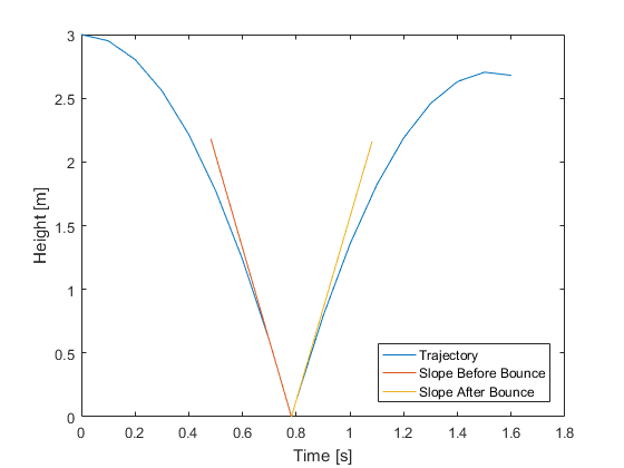
The second assumption is that the uncertainty stays centered on the state estimate during propagation. Remember in the sigma-point filter, we propagated each point separately, and then calculated a sample covariance at the end. That sample covariance was not necessarily still centered on the middle sigma point! EKFs, however, assume that it would be. This means that EKFs don't capture the nonlinearities of the propagation and measurement functions quite as well as sigma-point filters. It's part of the cost we pay for speed.

These assumptions are often acceptable even when not rigidly true, and this is one of the central themes in Kalman filtering: the assumptions are never rigidly true, but are often close enough to be useful.
Instead of trying to stay with the bouncing ball example, let's pick a more interesting example for the discussion of extended Kalman filters. It may be that, some day soon, when we order a small, light thing online, a little aircraft will spin up at a nearby distribution warehouse minutes later and fly it to our house, dropping it on a tiny parachute aimed approximately at our doorstep. Now when we wake up to find we're out of coffee filters, we can have them before we finish the morning jog. (The inclusion of the parachute is just to make sure nobody takes this example too seriously, and, really, why wouldn't we take the occassion to go to the neighborhood espresso shop?) So, our task will be to create a filter to watch the package go from the aircraft's location to the target drop location. For measurements, we'll again use position so that the plots will be easy to read.
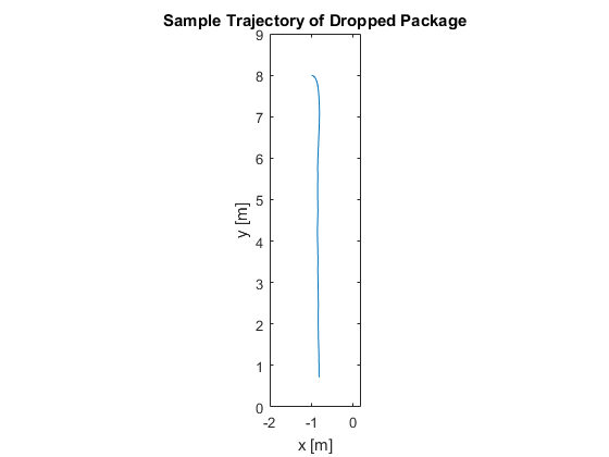
Before we begin, let's review some of the relevant symbols we've seen so far:
| Propagation and Prediction | |
|---|---|
| \(\hat{x}^+_{k-1}\), \(P^+_{k-1}\) | Corrected estimate and covariance from the last sample |
| \(f\) | Propagation function |
| \(Q\) | Covariance of the unknown process noise |
| \(\hat{x}^-_k\), \(P^-_k\) | Predicted estimate and covariance for this sample |
| \(h\) | Observation function |
| \(\hat{z}_k\) | Predicted measurement for this sample |
| Correction | |
| \(z_k\) | Measurement for this sample |
| \(R\) | Covariance of the unknown measurement noise |
| \(y_k\) | Innovation vector, \(z_k - \hat{z}_k\) |
| \(P_{xy}\) | State-innovation covariance |
| \(P_{yy}\) | Innovation covariance |
| \(K\) | Kalman gain |
| \(\hat{x}^+_k\), \(P^+_k\) | Corrected estimate and covariance for this sample |
Let's also take a quick look at the equations for one iteration of the extended Kalman filter, just to see what we're getting into (there's no need to understand them just yet):
$$ \begin{align} \hat{x}^-_k & = f(\hat{x}^+_{k-1}) \\ P^-_k & = F(\hat{x}^+_{k-1}) P^+_{k-1} F(\hat{x}^+_{k-1})^T + Q \\ \hat{z}_k & = h(\hat{x}^-_k) \\ P_{xy} & = P^-_k H(\hat{x}^-_k)^T \\ P_{yy} & = H(\hat{x}^-_k) P^-_k H(\hat{x}^-_k)^T + R \label{eq:Pyy} \\ K & = P_{xy} P_{yy}^{-1} \\ \hat{x}^+_k & = \hat{x}^-_k + K \left( z_k - \hat{z}_k \right) \\ P^+_k & = P^-_k - K H(\hat{x}^-_k) P^-_k \\ \end{align} $$This is often presented as either a recipe or as part of a rigid proof, and neither is very helpful for building intuition. Let's take it apart and see what we can do with it. Like all of the filters we're discussing, it starts with propagation.
Propagation
Extended Kalman filters, like sigma-point filters, represent uncertainty with a covariance matrix, but EKFs don't rely on sigma points in order to propagate that uncertainty. In fact, the propagation function is only used once: to propagate the last estimate to the time of the current measurement.
$$ \hat{x}^-_k = f(\hat{x}^+_{k-1}) $$(The little plus sign in \(\hat{x}^+_{k-1}\) means that it was the corrected estimate at \(k-1\), continuing the theme that \({}^-\) is used for predicted values and \({}^+\) for corrected values. So, the previous corrected state estimate is used to predict the current state.)
Also, we assume that the truth, \(x_{k-1}\), updates using the same function, plus some random process noise, \(q_{k-1} \sim N(0, Q)\) (“a random draw from a normal distribution with zero mean and covariance \(Q\)”), that represents random fluctations in the air that push the falling package around:
$$ x_k = f(x_{k-1}) + q_{k-1} $$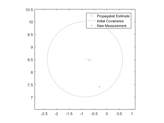
Without sigma points, how do we propagate the covariance, \(P^+_{k-1}\), to sample \(k\)? Since \(f\) is differentiable, we can calculate its Jacobian — its “slope”, in a matrix sense — and use that to propagate the covariance matrix directly. Let's see how.
Just like the slope of a one-dimensional function of \(x\) is the derivative of the function evaluated at some value of \(x\), the Jacobian matrix of the propagation function is the partial derivative of each element of the propagation function with respect to (wrt) each element of the state, evaluated at some value for the state. If \(F\) is the Jacobian matrix, and we wish to evaluate it at \(x_0\), then for each element \(i, j\) of \(F\):
$$ F_{i,j}(x_0) = \left. \frac{\partial}{\partial x_j} f_i \right\vert_{x_0} $$We usually write this more compactly for the whole matrix as simply:
$$ F(x_0) = \left. \frac{\partial}{\partial x} f \right\vert_{x_0} $$Recalling that \(Q\) is the process noise covariance matrix, the covariance can be propagated linearly from \(k-1\) to \(k\) as:
$$ P^-_k = F P^+_{k-1} F^T + Q $$where we've dropped the arguments to \(F\) for simplicity.
It's not immediately clear why this “propagates” the covariance, but it's actually pretty intuitive, once we recall what the Jacobian means and the definition of covariance. Let's start with the Jacobian.
If we know \(f(x_0)\), then we can approximate \(f(x_0 + \Delta x)\) for small \(\Delta x\) using a Taylor series expansion:
$$ f(x_0 + \Delta x) \approx f(x_0) + \left. \frac{\partial}{\partial x} f \right\rvert_{x_0} \Delta x + \ldots $$where the ellipsis stands for higher order terms, which can be ignored for small \(\Delta x\). Of course, \(\left. \frac{\partial}{\partial x} f \right\rvert_{x_0}\) is the Jacobian of \(f\), evaluated at \(x_0\).
Let's suppose that the true state is some small, hypothetical perturbation from our estimated state at \(k-1\):
$$ x_{k-1} = \hat{x}^+_{k-1} + \Delta x_{k-1} $$And, if we ignore process noise for just a moment, then the true state at \(k\) is:
$$ \begin{align} x_k & = f(x_{k-1}) \\ & = f(\hat{x}^+_{k-1} + \Delta x_{k-1}) \\ & \approx f(\hat{x}^+_{k-1}) + F \Delta x_{k-1} \end{align} $$Let's move \(f(\hat{x}^+_{k-1})\) to the left side:
$$ \begin{align} x_k - f(\hat{x}^+_{k-1}) & \approx F \Delta x_{k-1} \\ x_k - \hat{x}^-_k & \approx F \Delta x_{k-1} \\ \Delta x_k & \approx F \Delta x_{k-1} \\ \end{align} $$That's pretty plain. The Jacobian maps a perturbation at \(k-1\) to a perturbation at \(k\), to a first-order approximation. In fact, that's the meaning of the Jacobian. And since \(\Delta x_k\) is now approximated linearly, this process is called linearization.
Here's where the definition of covariance comes in: they're all about perturbations from a mean. Our perturbation above was just hypothetical, so if we think of it as a (zero-mean, Gaussian) random error in our state estimate, then the covariance of that error is just:
$$ P^+_{k-1} = E\left( \Delta x_{k-1} \Delta x_{k-1}^T \right) $$ $$ P^-_k = E\left( \Delta x_k \Delta x_k^T \right) $$Let's substitute the fact that we now know that \(\Delta x_k = F \Delta x_{k-1}\):
$$ P^-_k = E\left( F \Delta x_{k-1} \Delta x_{k-1}^T F^T \right) $$We can move \(F\) outside of the expectation:
$$ P^-_k = F E\left( \Delta x_{k-1} \Delta x_{k-1}^T \right) F^T $$and now we recognize \(P^+_{k-1}\) sitting in the middle there:
$$ P^-_k = F P^+_{k-1} F^T $$That is, the Jacobian just maps the \(\Delta x_{k-1}\) part on the left and the \(\Delta x_{k-1}^T\) part on the right to the future values. Easy.
For the last little touch, recall that we ignored the process noise. When the true state updates, the random process noise for that sample is added on:
$$ x_k = f(x_{k-1}) + q_{k-1} $$This is easy to account for, because we assumed that the process noise was uncorrelated with the state. The covariance of the sum of two uncorrelated random vectors is just the sum of the individual covariance matrices. So, we add \(Q\) on to the end, and now we have the form we were looking for:
$$ P^-_k = F P^+_{k-1} F^T + Q $$where the first part is the propagation due just to the dynamics around the mean (which may expand or contract), and the second part is due to the process noise (which always expands the covariance).
Putting it a different way: if a particle were located \(\Delta x\) away from the estimate, then it would propagate, to a first order approximation, as the estimate does, plus that little extra bit, \(F \Delta x\), and plus the process noise. The particles on all sides of the estimate would generally move outward, representing the growing uncertainty as time passes. We do all of this by simply calculating \(F\) and then using the equation above. Very compact.
Here are the results of our propagation of the state and covariance matrix:

Propagation, Redux
This article isn't about proofs; it's about intuition. If the propagation of the covariance matrix seems intuitive enough, then you might skip down to the next section and continue. However, if you'd like to run through the covariance propagation again, and build some intuition for the expectation stuff from above, then keep reading.
Instead of ignoring the process noise and tacking it on right at the end, let's consider it from the beginning. The propagation of the true state is actually this:
$$ x_k = f(x_{k-1}) + q_{k-1} $$Substituting in the perturbation we defined above:
$$ x_k = f(\hat{x}^+_{k-1} + \Delta x_{k-1}) + q_{k-1} $$Linearizing:
$$ \begin{align} x_k & \approx f(\hat{x}^+_{k-1}) + F \Delta x_{k-1} + q_{k-1} \\ & \approx \hat{x}^-_k + F \Delta x_{k-1} + q_{k-1} \\ \end{align} $$Moving the predicted state to the left:
$$ \begin{align} x_k - \hat{x}^-_k & \approx F \Delta x_{k-1} + q_{k-1} \\ \Delta x_k & \approx F \Delta x_{k-1} + q_{k-1} \\ \end{align} $$Using this to construct the covariance matrix, like before, we get:
$$ \begin{align} P^-_k & = E \left( \Delta x_k \Delta x_k^T \right) \\ & \approx E \left( (F \Delta x_{k-1} + q_{k-1}) (F \Delta x_{k-1} + q_{k-1})^T \right) \\ & \approx E \left( F \Delta x_{k-1} \Delta x_{k-1}^T F^T + F \Delta x_{k-1} q_{k-1}^T + q_{k-1} \Delta x_{k-1}^T F^T + q_{k-1} q_{k-1}^T \right) \\ \end{align} $$The expectation of the sum of different things is the sum of the expectation of each of those things:
$$ \begin{align} P^-_k \approx & E( F \Delta x_{k-1} \Delta x_{k-1}^T F^T ) \\ & + E( F \Delta x_{k-1} q_{k-1}^T ) \\ & + E( q_{k-1} \Delta x_{k-1}^T F^T ) \\ & + E( q_{k-1} q_{k-1}^T ) \\ \end{align} $$Recall that one of the assumptions of an extended Kalman filter is that the process noise at sample \(k-1\) is uncorrelated with the state at \(k-1\) (the state error doesn't affect the noise that gets generated). That's helpful, because the expected value of the product of two uncorrelated variables (their covariance) is 0 (remember the dice rolls above). So, the middle two terms in the above equation drop out. That leaves only:
$$ P^-_k \approx E(F \Delta x_{k-1} \Delta x_{k-1}^T F^T) + E(q_{k-1} q_{k-1}^T) $$\(F\) moves outside of the expectation operator:
$$ P^-_k \approx F E( \Delta x_{k-1} \Delta x_{k-1}^T ) F^T + E(q_{k-1} q_{k-1}^T) $$And we already have both of these quantities! The first is the covariance before the propagation, \(P^+_{k-1}\), and the second is the covariance of the process noise, \(Q\). We're back at the above form for the prediction of the covariance:
$$ P^-_k \approx F P^+_{k-1} F^T + Q $$While we've used the expectation operator here to make the meaning of this equation really clear, in practice, one most often uses the expectation operator when constructing the process noise covariance matrix, so it's a good thing to be comfortable with.
Correcting the Estimate
Now it's time to think about using the new measurement for correction. In fact, we can do this with pieces we've seen so far.
First, the Kalman gain and correction will be exactly the same as for the sigma-point filter.
$$ K = P_{xy} P_{yy}^{-1} $$ $$ \hat{x}^+_k = \hat{x}^-_k + K \left( z_k - \hat{z}_k \right) $$We just need to calculate the state-innovation covariance, \(P_{xy}\), and the innovation covariance, \(P_{yy}\). Let's start with the latter. We saw in the beginning of this section, \(\eqref{eq:Pyy}\), that the innovation covariance is given by:
$$ P_{yy} = H P^-_k H^T + R $$Notice how it has the same form as \(F P^+_{k-1} F^T + Q\)? That's because we'd derive it in exactly the same way, using the Jacobian of the observation function, \(H\), and the measurement noise covariance matrix, \(R\). The following is exactly the same as the derivation in the propgation section, with some of the letters swapped:
$$ \begin{align} z_k & = h(x_k) + r_k \\ z_k & = h(\hat{x}^-_k + \Delta x_k) + r_k \\ z_k & \approx h(\hat{x}^-_k) + H \Delta x_k + r_k \\ z_k & \approx \hat{z}_k + H \Delta x_k + r_k \\ z_k - \hat{z}_k & \approx H \Delta x_k + r_k \\ \Delta z_k & \approx H \Delta x_k + r_k \\ \end{align} $$Notice that \(\Delta z_k\) is the innovation vector, \(y\), but using the \(\Delta\) is a little clearer here. Its covariance tells us how much variability we expect in the difference between what we measure and what we predict as the measurement, so it represents both the error associated with our prediction and the error of the measurement itself.
We form the innovation covariance in exactly the same way we formed the propagated covariance (again just swapping some letters and noting that the measurement noise and estimate errors are uncorrelated):
$$ \begin{align} P_{yy} & = E \left( \Delta z_k \Delta z_k^T \right) \\ & = E \left( H \Delta x_k \Delta x_k^T H^T \right) + E \left( r_k r_k^T \right) \\ & = H E \left( \Delta x_k \Delta x_k^T \right) H^T + R \\ & = H P^-_k H^T + R \\ \end{align} $$So, just like \(F\) propagated a perturbation of the state from one time to another, \(H\) maps a perturbation of the state to a perturbation in the measurement. Then \(R\) joins in as extra measurement noise.
Forming the state-innovation covariance is even easier; we just plug things in and continue with the same themes:
$$ \begin{align} P_{xy} & = E \left( \Delta x_k \Delta z_k^T \right) \\ & = E \left( \Delta x_k \left( \Delta x_k^T H^T + r^T\right) \right) \\ & = E \left( \Delta x_k \Delta x_k^T \right) H^T + E \left( \Delta x_k r^T \right) \\ & = E \left( \Delta x_k \Delta x_k^T \right) H^T + 0 \\ & = P^-_k H^T \\ \end{align} $$So, \(P_{xy}\) just represents a perturbation in the estimate “on the left” with a perturbation in the predicted measurements “on the right”. Since the measurement noise and predicted measurement are uncorrelated (it's the term that's cancelled in the fourth line, above), the measurement noise covariance, \(R\), doesn't show up in \(P_{xy}\) at all.
Recall how we constructed \(P_{xy}\) for the sigma point filter: we calculated the sample covariance of the sigma points, using the difference in each sigma point from the mean in state space on the left, and the difference in the predicted measurement from the mean on the right. That's exactly what we're doing here, but in matrix fashion, to a first-order approximation.
All of this first-order approximation stuff should make it clear why an extended Kalman filter is a linear filter, even when it's applied to a nonlinear problem.
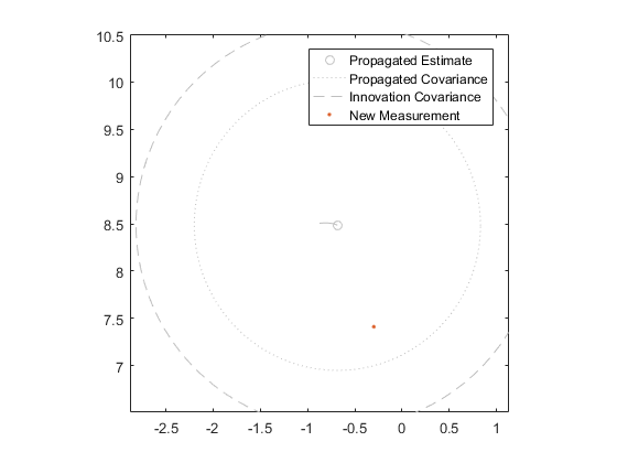
With the state-innovation covariance matrix and innovation covariance matrix in place, we can calculate the Kalman gain and update the state estimate, as before.
Correcting the Covariance
There's only one thing left: how do we update the covariance matrix to account for this correction? We stated at the very beginning that the correction is:
$$ P^+_k = P^-_k - K H P^-_k $$But why? That's not even symmetric! What is going on here?
Let's think back to sigma-point filters again. There, we said we could update each sigma point individually; each would therefore converge towards the measurement to some degree, and that convergence towards a single point represented the shrinking of the covariance matrix. Well, a sigma point is like a little \(\Delta x\) from the mean, so let's make the updated covariance matrix with some corrected little perturbations.
We've already used \(\Delta x_k\) as the perturbation of the truth from the predicted state, \(\hat{x}^-_k\), so let's use \(\Delta x^+_k\) as the perturbation of the truth from the corrected estimate, \(\hat{x}^+_k\):
$$ x_k = \hat{x}^+_k + \Delta x^+_k $$And we'll restate what the corrected estimate is:
$$ \hat{x}^+_k = \hat{x}^-_k + K (z_k - \hat{z}_k) = \hat{x}^-_k + K \Delta z_k $$Let's plug them in.
$$ \begin{align} \Delta x^+_k & = x_k - \hat{x}^+_k \\ \Delta x^+_k & = x_k - \left( \hat{x}^-_k + K \Delta z_k \right) \\ \Delta x^+_k & = x_k - \hat{x}^-_k - K \Delta z_k \\ \Delta x^+_k & = \Delta x_k - K \Delta z_k \\ \end{align} $$No surprise here: the corrected perturbation is slightly smaller than the original perturbation by the amount of the correction. So what's the covariance of this thing? As is now the usual procedure, we'll just start from the definition of the covariance, plus things in, move the expectation operators around a bit, and cancel anything we can.
$$ \begin{align} P^+_k = & E \left( \Delta x^+_k {\Delta x^+_k}^T \right) \\ = & E \left( \left( \Delta x_k - K \Delta z_k \right) \left( \Delta x_k - K \Delta z_k \right)^T \right) \\ \end{align} $$Skipping the multiplication and moving the expectation operator around, which we've done many times now:
$$ \begin{align} P^+_k = & E \left( \Delta x_k \Delta x_k^T \right) \\ & - E \left( \Delta x_k \Delta z_k^T \right) K^T \\ & - K E \left( \Delta z_k \Delta x_k^T \right) \\ & + K E \left( \Delta z_k \Delta z_k^T \right) K^T \\ \end{align} $$Recalling that \(P_{xy} = E \left( \Delta x \Delta z_k^T \right) \) and \(P_{yy} = E \left( \Delta z_k \Delta z_k^T\right) \), we can substitute:
$$ P^+_k = P^-_k - P_{xy} K^T - K P_{xy}^T + K P_{yy} K^T$$That's a little better. It's symmetric, like we'd expect (no pun intended) for a covariance operation. Also, we haven't made any assumptions on \(K\). This is actually general for any \(K\). But we care about the Kalman gain, so let's substitute in the Kalman gain in just one location near the end:
$$ P^+_k = P^-_k - K P_{xy}^T - P_{xy} K^T + \left( P_{xy} P_{yy}^{-1} \right) P_{yy} K^T $$Since \(P_{yy}^{-1} P_{yy}\) is an identity matrix, we can drop it:
$$ P^+_k = P^-_k - K P_{xy}^T - P_{xy} K^T + P_{xy} K^T $$The two right terms cancel out:
$$ P^+_k = P^-_k - K P_{xy}^T $$And now we just substitute \(P_{xy} = P H^T\):
$$ \begin{align} P^+_k & = P^-_k - K \left( P^-_k H^T \right)^T \\ & = P^-_k - K H P^-_k \\ \end{align} $$And there it is! There's no magic here; it's just the same old process: express things in terms of perturbations, set up the covariance definition, move things around, and cancel stuff. And now that we know the \(K\) is constructed so that this actually is symmetric and makes sense, we can see the simple meaning of this equation: the Kalman gain tells us how much of our current covariance we can subtract off thanks to the most recent measurement. Large Kalman gains correspond to low measurement noise (measurement noise is part of \(P_{yy}\), which is the “denominator”), and so when measurement noise is low, we can subtract off a lot of our current uncertainty. When measurement noise is high, the gain will be small, so we won't subtract off very much.
Correction, Redux
That was a lot of material, but each step was actually pretty small: just some matrix multiplication, a few assumptions, and the expectation operator. That's really all it takes to work with these (it takes a little more to do proofs about why the Kalman gain is particularly good). Let's wrap up this discussion of the extended Kalman filter's correction process with another animation, using some example values. We'll put the state stuff in the left plot and the measurement stuff in the right plot. We start with the state estimate (0, 0) and the covariance, shown with a bunch of particles.
- We map the state estimate to the predicted measurement.
- We map the covariance in the state (all those particles) to observation space too. (This is like \(H P^-_k H^T\).)
- We then add on the measurement noise, \(R\). This gives us \(P_{yy} = H P^-_k H^T + R\). We see this as an increase in the distribution of the particles in observation space.
- The actual measurement comes in.
- (We show how well each particle predicted the measurement.)
- (We color the corresponding particles in state space too.)
- The Kalman gain is calculated, and we plot the corrected state. Not surprisingly, it sits pretty well within the most likely particles.
- The covariance is corrected, seen here as a correction in each particle. They clearly move closer together around the corrected estimate.
- (We use those corrected particles to predict the observation again, just for fun. Look how they move right over towards the measurement, but not quite all the way to it.)
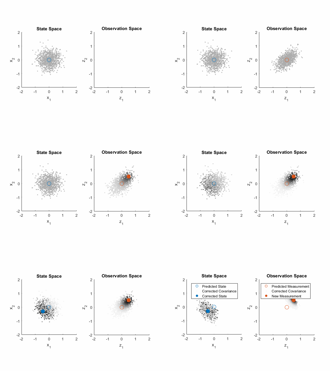
That completes the extended Kalman filter! Every step of the process is actually fairly intuitive, once we have a good grasp of:
- first-order approximations of nonlinear functions,
- the definition of covariance,
- and the meaning of “uncorrelated” random variables.
Finally, here's the corrected estimate and covariance for our falling coffee filters:

By repeating the overall process every time we get a new measurement, we can often converge on good estimates very quickly, with just one call to \(f\) and \(h\) per measurement and a little matrix math. Here are the results for our coffee filter delivery:

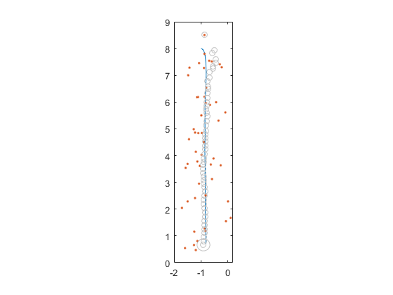
Outline of an Extended Kalman Filter
- Calculate the Jacobian of the propagation function and the process noise covariance matrix.
- Propagate the state.
- Propagate the estimate covariance.
- Predict the measurement.
- Calculate the Jacobian of the observation function and the measurement noise covariance matrix.
- Calculate the Kalman gain.
- Correct the estimate and its covariance matrix.
Steps 4 through 7 correspond to the animation above.
Assumptions, Advantages, and Disadvantages
The extended Kalman filter makes more assumptions about the problem than the sigma-point filter, and so is slightly less general. Those assumptions are:
- The functions are smooth.
- The covariance remains centered on the propagated state.
- The linear approximations are sufficiently accurate for the changes to the covariance matrix over time.
- The process noise, measurement noise, and estimate errors are Gaussian and uncorrelated.
Where their assumptions approximately apply, extended Kalman filters are a great option. Indeed, they are the workhorse of state estimation in many industries and in many forms. The advantages are:
- They apply well to many smooth problems.
- They're fast.
- They're very well studied and have many great options for detailed implementations.
The primary disadvantages of EKFs are:
- Creating analytical Jacobians is not always feasible. In these cases, a sigma-point filter should probably be used instead.
- The Jacobians are constructed from estimates. If the estimates are too far from the truth, the Jacobians will be wrong, and the corrections therefore might not ever converge on the truth (they may even be worse than the observations themselves). This is called divergence. We'll see some strategies for dealing divergence in part 2.
Before we go into these options and implementation details, we have one more filter architecture to cover: the Kalman filter.
The Kalman Filter
We finally arrive at Kalman's original algorithm for state estimation of linear systems. For linear systems, the propagation and observation functions are expected to look something like this:
$$ x_k = F x_{k-1} + F_u u_{k-1} + q_{k-1} $$ $$ z_k = H x_k + H_u u_k + r_k $$where \(F\), \(F_u\), \(H\), and \(H_u\) are the system matrices and \(u\) is some input vector, which can contain anything that linearly affects the propagation (control inputs, gravity, biases). It's assumed to be known. Of course, \(F\) and \(H\) mean the same thing as before.
Of course, nobody's problem is actually a linear system (they're like perfect vaccuums or point masses — pleasant idealizations). Further, the linear Kalman filter is just a special case of the extended Kalman filter, so why would we bother learning about it? Because linear filters are very often useful on nonlinear problems. In fact, we'll recast our falling coffee filters filter above as a linear filter with virtually no loss in performance.
The key to linear filtering is to use error states — states that represent small deviations from some nominal state. For instance, our package has a parachute and quickly reaches its terminal velocity, where the forces due to drag and gravity cancel. Let's call this our nominal velocity, and we can arbitrarily pick the target landing site (0, 0) as the nominal position. So, our nominal state is \(x_n = \begin{bmatrix} 0 & 0 & 0 & -v_t \end{bmatrix}^T\), where \(v_t\) is the terminal velocity (by the end, the velocity will nominally be downward). Our error state is just the truth minus this nominal state:
$$ \Delta x = x - x_n $$Let's linearize the dynamics of this deviation near the nominal state.
$$ \begin{align} \Delta x_k & = x_k - x_n \\ & = f(x_{k-1}) - x_n \\ & = f(x_n + \Delta x_{k-1}) - x_n \\ & \approx f(x_n) + F \Delta x_{k-1} - x_n \\ \end{align} $$Note that both \(x_n\) and \(f(x_n)\) are constants, so let's set \(\Delta x_n = f(x_n) - x_n\). The resulting model is clearly linear, following the form above, where \(\Delta x_n\) is the input vector (\(u_{k-1}\) in the above), and the input map (\(F_u\) above) is the identity matrix.
$$ \Delta x_k = F \Delta x_{k-1} + \Delta x_n $$Of course, the observation function needs to be linear too, but this is trivial for our simple problem:
$$ z_k = \begin{bmatrix} 1 & 0 & 0 & 0 \\ 0 & 1 & 0 & 0 \end{bmatrix} \Delta x_k $$(If it had been a more difficult function, we would have gone through the same type of linearization that we did for the propagation portion.)
Otherwise, the only remaining parts are the process and measurement noise covariance matrices, and they're exactly the same whether we deal with full states or deviations. We're ready to filter just like we did before. Here are the results for the package delivery:
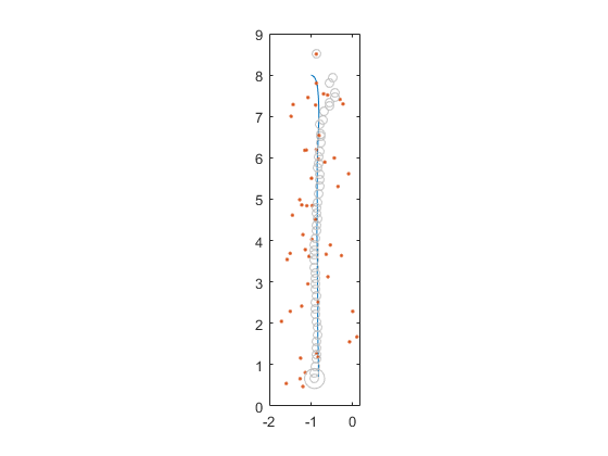
There's no noticeable difference from the extended filter. Let's look at the state estimates individually, and at the difference between the extended and linear Kalman filter estimates.
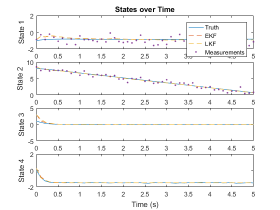
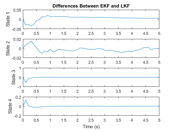
There's a small difference, not surprisingly at the beginning, when the package isn't yet at terminal velocity, but it's negligible compared to the overall accuracy of the filters. This is pretty common. There are many nonlinear problems that can be estimated quite well using a fully linear filter. This enables the filter to run extra quickly, as there's no need to re-calculate the Jacobians over time or run detailed propagation and observation functions. The key to building a linear filter is to find a good nominal point or nominal trajectory along which the Jacobians are constant. This can't be done for all problems, but it's a great technique when it can be done, and it's often needlessly overlooked.
Steady-State Covariance
There's an interesting thing to note for Kalman filter: since \(F\), \(H\), \(Q\), and \(R\) are constant, the state does not affect the covariance. Let's take a look at the code that would update the covariance in a linear Kalman filter:
P = F * P * F.' + Q;
K = P * H / (H * P * H.' + R); % The / is a matrix inverse here.
P = P - K * H * P;
Nothing here requires the state! The progression from the initial covariance to a steady-state value can be entirely predicted ahead of time, before actually running the filter. And once the covariance matrix reaches a steady state, there's no point in continuing to update it. After that point, the Kalman gain is constant. As an extreme case, if it would be reasonable to initialize a filter with the steady-state covariance, then one could instead calculate the Kalman gain associated with the steady-state covariance ahead of time and implement a filter that never needs the covariance at all, such as:
x     = F * x + F_u * u;
z_hat = H * z + H_u * u;
x     = x + K * (z - z_hat); % K is constant!
This steady-state form is actually called a Wiener filter, after Dr. Norbert Wiener at MIT, whose work predated Kalman's by about a decade.
Without the need to calculate the Kalman gain in the loop, or to store any of the covariance matrices, this is a very lightweight filter that nonetheless has the advantages of a Kalman filter. Again, it only applies when the initial uncertainty is the steady-state value and the system matrices are constant, but in such a case, it can't be beat.
Outline of a Linear (Discrete) Kalman Filter
- Propagate the state.
- Propagate the covariance.
- Predict the measurement.
- Calculate the Kalman gain.
- Correct the state and covariance.
Wrap-Up
We've looked at four filter architectures and discussed how they all do similar things with different assumptions, which enable different operations, which enable differences in accuracy and speed.
- Particle filters are very general and are a common choice when the probability density is multimodal. They work well enough when runtime isn't a concern.
- Sigma-point filters use a small set of “particles” placed on an ellipsoid around the state estimate. They therefore assume that the probability density is unimodal. They also assume that the process and measurement noise are uncorrelated with each other and with the state. They're substantially faster than particle filters, and they handle nonlinearities better than extended Kalman filters.
- Extended Kalman filters assume that the propagation and observation functions are smooth and that the covariance propagates linearly and stays centered on the propagated estimate, in addition to all of the assumptions made by sigma-point filters. They're fast and have some options (in the next part) for being very fast. They also have a long history of working well even on problems that violate their assumptions to startling degrees, so EKFs are a great option to try for a wealth of state estimation problems.
- Linear Kalman filters are the same as extended Kalman filters, but (usually) propagate error states with approximately linear dynamics. They're a little faster, and the simplified code works well for embedded systems.
There are many different types of state estimators, and many variations on each, but these four represent the basics of how estimates and uncertainty are propagated and updated sequentially as new measurements become available.
But we're not done. When the extended Kalman filter was created for the Apollo program, it was coded up as part of a simulation of the spacecraft, and after one small bug fix, it worked well. The engineers on Apollo could have stopped here; most people declare success as soon as they see decent results in simulation. The Apollo folks, however, went forward and found that there were several more things that were necessary before the filter was practical and reliable. In fact, they discovered, the “default” Kalman filter algorithm above is poorly suited to implementation in computers! Fortunately, a few tweaks enable it to:
- run very, very quickly,
- maintain stability despite the potential for build-up of roundoff errors,
- and estimate more accurately.
In the next part, we'll see how these are relatively easy modifications once one has an understanding of how the filters actually work.
References
The sample code includes a particle filter, sigma-point filter, extended Kalman filter, and linear Kalman filter, as well as some utilities and the files used to generate the plots for this article. It's available here.
Probabilistic Robotics by Thrun, Burgard, and Fox contains entry-level material for particle filters and sigma-point filters and discusses their use in robot location-finding (a multimodal problem where particle filters have proven useful, even in embedded applications).
Kalman Filtering and Neural Networks, edited by Haykin, provides great information about the unscented Kalman filter (sigma-point filter) and is frequently cited in the literature. It includes numerous practical forms, with accessible discussion and very good pseudocode.
Estimation with Applications to Tracking and Navigation by Bar-Shalom, Li, and Kirubarajan is probably the single best book on extended Kalman filtering, whether one is interested in tracking or not, and it includes advanced implementation options for speed and stability. However, it's a theory-heavy book and can go very slowly until one understands some of the subtlety of probability theory.
Greg Welch and Gary Bishop maintain this page for information on Kalman filtering and many related things. It's a good resource.
The various IEEE journals and the AIAA Journal of Guidance, Control, and Dynamics provide numerous excellent papers on practical filters with pseudocode, simulations, and discussions of results from real-world testing. Of course, these are generally industry-specific. No book even comes close to the depth available from the journals.
Fragments of the story of the development of the Kalman filter for the Apollo program are scattered all over. However, NASA maintains a brief and enjoyable write-up by Leonard A. McGee and Stanley F. Schmidt called “Discovery of the Kalman Filter as a Practical Tool for Aerospace and Industry”, located here. Another much more modern write-up is “Applications of Kalman Filtering in Aerospace 1960 to the Present” by Grewal (who runs a class on Kalman filtering for GPS and IMUs) and Andrews.