Useful Little Things
There are a lot of little mathy things that go into building filters and related simulations. We'll go over some of the most useful things, with just enough math to make it clear that there's no magic here and to practice the ideas from the first two parts. This part goes a little more quickly than the previous two, with the math generally functioning as exercises for things we've already seen.
Random Draws from a Covariance Matrix
When simulating filters, or even inside some filters themselves (like the bootstrap filter), one needs to take random draws with a certain covariance, which we'll call \(Q\). It's not immediately clear how to do this, so let's start with what we have: any relevant programming language has libraries for generating random numbers/vectors with a Gaussian distribution and unit variance.
For instance, in MATLAB we can generate a single random vector with x1 = randn(3, 1);, and we can generate 1000 random vectors all at once with:
x = randn(3, 1000); % a 3-by-1000 matrix
The randn function produces random numbers with unit variance, meaning:
where \(I\) is an identity matrix. (In languages that are not matrix-oriented, we can fill a 2D array with independent draws from a 1-dimensional Gaussian random number generator, and then we'll have the same thing.)
We want the covariance to be \(Q\). How? Let's use some of the same matrix decomposition stuff we used in the square-root filter section: the Cholesky factor. We can calculate some matrix, \(C\), so that:
$$ Q = C C^T $$Now let's see what the covariance of \(C x\) is.
$$ E(C x x^T C^T) = C E(x x^T) C^T $$We saw above that the middle part is an identity matrix, so:
$$ \begin{aligned} E(C x x^T C^T) & = C E(x x^T) C^T \\ & = C I C^T \\ & = C C^T \\ & = Q \end{aligned} $$So, to obtain random draws with covariance, \(Q\), we start with random draws with unit variance, then multiply them by the Cholesky factor of \(Q\). Here it is as MATLAB code:
C = chol(Q, 'lower'); % Make sure to use *lower* Cholesky factor!
x = randn(nx, n);     % Make n random nx-dimensioned vectors.
y = C * randn(nx, n); % Give them the proper covariance.
As a final detail, note that we said in the first part the covariance matrices must be positive-semidefinite (\(z^T P z \geq 0\)), but Cholesky decomposition only works on strictly postive-definite matrices (\(z^T P z \gt 0\)). So, there are actually better ways to calculate \(C\) that work even in semidefinite cases. We can use singular value decomposition (SVD) for this, which breaks a matrix, \(Q\), down into three parts, \(U\), \(S\), and \(V\), so that:
$$ Q = U S V^T $$where \(S\) has values only on the diagonal, and they're all positive (or 0). When performed on a covariance matrix, it turns out that \(U = V\), so \(Q = U S U^T\).
Because \(S\) only has values on the diagonal, calculating its square root, \(S^{1/2}\), is easy: we just take the square root of each value individually. We can then construct \(C\):
$$ C = U S^{1/2} $$Just to check:
$$ C C^T = U S^{1/2} {S^{1/2}}^T U^T = U S U^T = Q $$Let's revise the code:
[U, S] = svd(Q);      % Works even when Q is positive-semidefinite.
C = U * sqrt(S);      % Construct the matrix square root.
x = randn(nx, n);     % Make n random nx-dimensioned vectors.
y = C * randn(nx, n); % Give them the proper covariance.
Ellipses from Covariance Matrices
It's sometimes useful to actually draw covariance matrices as ellipsoids, and this is surprisingly easy to do with the fundamentals we have already. First, let's acknowledge that a unit circle is the 1σ boundary for a unit normal distribution, by definition. And we know that if we multiply points from a unit normal distribution by \(C\), we can obtain some other distribution, just as we saw above. The matrix \(C\) maps points from the unit distribution to another distribution. For exactly the same reason, it would map the points of the 1σ circle for the unit distribution to the 1σ circle of the desired distribution. The code is easy:
[U, S]  = svd(P);                   % SVD of relevant dimensions of P
C       = U * sqrt(S);              % Form matrix square root.
theta   = linspace(0, 2*pi, 100);   % Make 100 points from 0 to 2*pi.
circle  = [cos(theta); sin(theta)]; % Make a unit circle.
ellipse = C * circle;               % Map points of circle to ellipse.
In the case of the bouncing ball, where we drew the ellipse over time, we calculated the ellipses corresponding to the position parts of the covariance matrix (indices 1 and 2, or P(1:2, 1:2)).
Naturally, if we want the ellipse centered somewhere, like on a state estimate, we add the location to each element of the ellipse.
Creating Random Covariance Matrices
It can be useful to create random covariance matrices in order to test algorithms, and this too is easy now that we're familiar with matrix decomposition. We know that a valid covariance matrix must break down into \(U\) and \(S\), where \(S\) is diagonal and only has positive values (or zeros), so all we need to do is generate random values for these. The trick is that \(U\) must be unitary for this to make sense (its inverse is its transpose). Since SVD gives us a unitary matrix, we'll use SVD on a random matrix to get a random unitary matrix (there are faster ways, but this is already pretty fast).
% Make some random singular values (or eigenvalues -- same thing!)
% from 0 to 1, or we could set a minimum and maximum.
s = rand(1, n);

% Make a matrix of n-by-n random numbers.
A = randn(n);

% Use SVD to get a random unitary matrix.
[U, ~, ~] = svd(A); % The ~ means we throw away the S and V parts.

% Make the covariance matrix.
P = U * diag(s) * U.';
Discretization
We're using discrete-time filters, but very often the underlying dynamics are better expressed in continuous time, such as for position and velocity:
$$ \dot{x} = f_c(x) $$Further, it's generally far easier to calculate the Jacobians of the continuous-time expression:
$$ F_c = \left. \frac{\partial}{\partial x} f_c \right|_{x_0} $$However, we need the Jacobians of the discrete dynamics:
$$ x_k = f(x_{k-1}) $$ $$ F = \left. \frac{\partial}{\partial x} f \right|_{x_0} $$What do we do in this case? Fortunately, we can convert from continuous time to discrete time. The best way to do this is with a matrix exponential:
$$ F \approx e^{F_c \Delta t} $$where \(\Delta t\) is the time step of the discrete system. In fact, when the system is linear, this conversion is exact.
Matrix exponentials are expensive. When this operation can be performed once, offline, then that's no concern, but when it must be performed inside the filter (such as for extended Kalman filters), we might seek a simpler form. For instance, we might update position as velocity times the time step, and velocity as acceleration times the time step (we ignore the direct effect of acceleration on position for small time steps). This is rough, but is sometimes acceptable when the time step is very small. Expressing this in matrix form, we'd have:
$$ F \approx I + F_c \Delta t $$where \(I\) is an identity matrix. (See the beginning of “How Simulations Work” to see what can go wrong with the “just multiply by \(\Delta t\)” method.)
Another possibility is the bilinear or Tustin transform:
$$ F \approx \left( I + \frac{1}{2} F_c \Delta t \right) \left( I - \frac{1}{2} F_c \Delta t \right)^{-1} $$There's a matrix inverse, which is usually expensive, but in practice, \(I - \frac{1}{2} F_c \Delta t \) often has a block structure that can be inverted with a series of smaller (even trivial) inversions using block matrix inversion.
What about the other Jacobians? Sometimes there's a Jacobian for the input vector, \(u\) (for linear Kalman filters), and for the process noise, \(q\). The linearized dynamics would look something like this:
$$ \dot{x} = F_c x + F_{c,u} u + F_{c,q} q $$Due to the way they interact with the state, these must all be discretized together. This is actually no harder than before, but first we need to change the way we look at the problem. Consider an “augmented” state:
$$ x_a = \begin{bmatrix} x \\ u \\ q \end{bmatrix} $$The \(u\) and \(q\) vectors are considered constant over the time step for discrete filters, so their time-derivatives are zero within the time step. So we can easily construct the derivative of the augmented state:
$$ \dot{x}_a = \begin{bmatrix} \dot{x} \\ 0 \\ 0 \end{bmatrix} = \begin{bmatrix} F_c & F_{c,u} & F_{c,q} \\ 0 & 0 & 0 \\ 0 & 0 & 0 \\ \end{bmatrix} \begin{bmatrix} x \\ u \\ q \end{bmatrix} = F_{c,a} x_a $$where those zeros have the appropriate dimensions.
Now let's discretize the augmented system (we could use any method from above, but we'll stick with the matrix exponential):
$$ F_a = e^{F_{c,a} \Delta t} = \begin{bmatrix} F & F_u & F_q \\ 0 & I & 0 \\ 0 & 0 & I \\ \end{bmatrix} $$And the discrete versions of the Jacobians are sitting along the top.
This works with the bilinear transform too, and, using the properties of block matrix inversion, we would only need to calculate the top row.
Setting Up Covariance Matrices
There are usually three covariance matrices we need to set up for a filter: the initial covariance, the process noise covariance, and the measurement noise covariance.
Measurement Noise Covariance
The simplest of these is usually the measurement noise covariance matrix. This often consists of values taken directly from sensors' specification sheets, and the errors are usually uncorrelated. In this case, this matrix would be constructed by simply placing the relevant values on the diagonal. For instance, if the specification sheets reported the standard deviations (\(\sigma_1\), \(\sigma_2\), ...) of the errors, then the measurement noise covariance might look like this:
$$ R = \begin{bmatrix} \sigma_1^2 & 0 & \ldots & 0 \\ 0 & \sigma_2^2 & \ldots & 0\\ \vdots & \vdots & \ddots & \vdots \\ 0 & 0 & \ldots & \sigma_n^2 \\ \end{bmatrix} $$Initial Estimate Covariance
The initial estimate covariance matrix is commonly set in one of two ways. The first is a simple diagonal matrix with the squares of the standard deviations of the state on the diagonal. This implies that no covariance is initially known.
$$ P_0 = \begin{bmatrix} \sigma_1^2 & 0 & \ldots & 0 \\ 0 & \sigma_2^2 & \ldots & 0\\ \vdots & \vdots & \ddots & \vdots \\ 0 & 0 & \ldots & \sigma_n^2 \\ \end{bmatrix} $$The second way is used when the initial state is created from an initial measurement. In this case, the measurement noise covariance matrix will be used as part of, all of, or to inform the initial covariance. For instance, if we measured position but not velocity, the initial estimate might be the measured position and zero velocity. The covariance would be the measurement covariance (let's call it \(R\)) for the position terms and independent velocity terms:
$$ P_0 = \begin{bmatrix} R & 0 \\ 0 & P_{vv} \\ \end{bmatrix} $$Otherwise, when some initial covariance is known, one should of course try to use it. This will look different for every problem.
Process Noise Covariance
Usually, the most difficult covariance matrix to set up is the process noise. Let's continue with our position-velocity examples.
$$ x = \begin{bmatrix} r_1 \\ r_2 \\ v_1 \\ v_2 \end{bmatrix} $$where \(r\) denotes “position” and \(v\) denotes “velocity”. Let's suppose that the process noise is a random acceleration (\(a_1\) and \(a_2\)), held constant over the time step. Acceleration maps to velocity as \(\Delta t\) and to position as \(\frac{1}{2} \Delta t^2\), so the effect of the random acceleration is:
$$ x_k = f(x_{k-1}) + F_a \begin{bmatrix} a_1 \\ a_2 \end{bmatrix} $$where
$$ F_a = \begin{bmatrix} \frac{1}{2}\Delta t^2 & 0 \\ 0 & \frac{1}{2}\Delta t^2 \\ \Delta t & 0 \\ 0 & \Delta t \\ \end{bmatrix} $$If the covariance of \(a\) is \(Q_a\), then what's the covariance of \(q = F_a a\)?
$$ \begin{align} Q & = E \left( F_a a a^T F_a^T \right) \\ & = F_a E \left( a a^T \right) F_a^T \\ & = F_a Q_a F_a^T \end{align} $$We can now express the update of the true state in terms of this “effective” process noise:
$$ x_k = f(x_{k-1}) + q_{k-1} $$where \(q_{k-1} \sim N(0, Q)\). This is the form we need for a Kalman filter, so we'd use \(Q\) as the process noise covariance matrix in the filter.
If there were more noise sources, we'd continue with this type of development for each. For instance, suppose there were some other random noise, \(b\), acting on the state.
$$ x_k = f(x_{k-1}) + F_a a + F_b b $$The effective noise is \(q = F_a a + F_b b\). What's the covariance of it?
$$ \begin{align} Q & = E \left( q q^T \right) \\ & = E \left( \left(F_a a + F_b b\right) \left(F_a a + F_b b\right)^T \right) \\ \end{align} $$After multiplying out and pulling constants out of the expectation:
$$ \begin{align} Q = & F_a E \left( a a^T \right) F_a^T \\ & + F_a E \left( a b^T \right) F_b^T \\ & + F_b E \left( b a^T \right) F_a^T \\ & + F_b E \left( b b^T \right) F_b^T \\ \end{align} $$If those noise sources are uncorrelated, then \(E\left(a b^T\right)\) is 0, so the middle two terms above drop out.
$$ \begin{align} Q & = F_a E \left( a a^T \right) F_a^T + F_b E \left( b b^T \right) F_b^T \\ & = F_a Q_a F_a^T + F_b Q_b F_b^T \\ \end{align} $$Not surprisingly, the covariance matrices of uncorrelated noise sources add.
Creating process noise covariance matrices for realistic problems generally uses the techniques here and in the discretization section. A normal procedure might look like:
- Set up the definition of the effective process noise in terms of whatever is known from first principles.
- Multiply. This is usually a mess of subscripts and transposes.
- Cancel out the covariance of uncorrelated terms, which usually simplifies the above dramatically.
- Find “small” things that can be ignored.
- Discretize, where appropriate.
Likelihood of a Given Error
In particle filters, we needed to be able to answer the question, “How likely is it that we'd see an error this big?“ For instance, suppose our error is \(\Delta z = \begin{bmatrix} 1.2 & 0.4 \end{bmatrix}\) and that the measurement error is Gaussian, with zero mean and covariance \(R\). How likely is \(\Delta z\)? Note that we aren't looking for the chances that an error will be exactly \(\Delta z\), because the chances of any particular error are infinitessimally small. (What are the chances that a random number generator will generate exactly 1.2? Pretty much 0.) What we want to know is what the probability density is at \(\Delta z\) from the mean.
The probability density function (PDF) for a multivariate distribution with covariance \(R\) is:
$$ \frac{1}{\sqrt{\left( 2 \pi \right)^n \left|R\right|}} e^{-\frac{1}{2} \Delta z^T R^{-1} \Delta z} $$where \(n\) is the dimension of \(\Delta z\) and \(\left|R\right|\) is the determinant of \(R\).
The PDF is undefined if \(R\) is indefinite (the determinant would be 0). That would be like asking how likely an error is when an error is impossible.
For other distributions, probability density functions can be found in a probability textbook or on Wikipedia.
Checking for Positive-Definiteness
Sometimes we just need to check to see if a matrix is positive-semidefinite. This ultimately means that the eigenvalues should be greater than or equal to zero. To see why, let's remember what eigenvalue and eigenvectors are (and skip down to the code, below, if you don't care to see why, but it's instructive, because people so frequently talk about the eigenvalues of covariance matrices).
If \(D\) is a matrix with the eigenvalues of \(P\) arranged on the diagonal, and \(V\) is a matrix whose columns are the corresponding unit eigenvectors, then:
$$ P V = V D $$If \(P\) is symmetric, as it must be, then each eigenvector will be orthogonal to all other eigenvectors (this a property of eigenvectors for symmetric matrices), meaning that, if \(v_i\) and \(v_j\) are two of the eigenvectors (columns) from \(V\), then their inner product, \(v_i^T v_j\), is 1 when \(i = j\) (they're the same vector) and 0 otherwise. That means \(V^T V = I\), an identity matrix, which means \(V^T\) is the inverse of \(V\). So we have:
$$ P V V^T = P = V D V^T $$If \(P\) were to be indefinite, then \(a^T P a \lt 0\) for some \(a\).
$$ a^T P a = a^T V D V^T a \lt 0 $$Of course, \(a' = V^T a\) is just some new vector, and \(a\) is arbitrary anyway, so this is equivalent to:
$$ {a'}^T D a' \lt 0 $$where now \(a'\) is arbitrary. And, since \(D\) is diagonal, this simplifies to:
$$ {a'}^T D a' = {a'}_1^2 D_{1,1} + {a'}_2^2 D_{2,2} + \ldots + {a'}_n^2 D_{n,n} \lt 0 $$Those squared values from \(a'\) certainly aren't negative, so the only way it's possible that this sums to less than 0 is if some of the values of \(D\) are less than zero. Further, if any value of \(D\) were negative, say \(D_i\), then we could just pick \(a'\) so that it would be zero everywhere except for \({a'}_i\) (because it's arbitrary). Then the sum would be just \({a'}_i^2 D_{i,i}\), which would clearly be less than zero if \(D_{i,i}\) were less than 0. So, the necessary and sufficient condition for checking \(P\)'s positive-definiteness is that the eigenvalues are greater than or equal to zero. We never actually need the eigenvectors! The code:
positive_definite     = all(eig(P) > 0);
positive_semidefinite = all(eig(P) >= 0);
Eigenvalue-eigenvector decomposition is slower than some other methods and is clumsy (what if \(P\) isn't perfectly symmetric? what if an eigenvalue ends up imaginary?), so there are better methods. For instance, recall \(U D U^T\) decomposition from the “square-root filter” section.
$$ U D U^T = P $$Again, due to the arbitrariness of picking the \(a\) vector, the \(U\) matrices don't matter, and we can just check that all of the diagonals of \(D\) are positive for positive-definiteness (or greater than or equal to zero for positive-semidefiniteness).
[~, d] = udfactor(P); % d is a *vector* of the diagonals
positive_definite     = all(d > 0);
positive_semidefinite = all(d >= 0);
We could have started with \(UDU^T\) factorization, but it's more common to speak of the eigenvalues of a covariance matrix than any other decomposition, so this was good practice.
Random Draws from a Discrete Probability Distribution
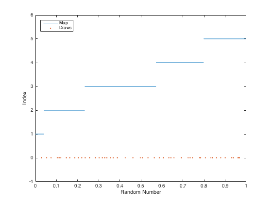
When randomly selecting particles according to their weights, the weights act as a probability mass function, or discrete probability distribution. When implemented as an algorithm, the input is the set of weights, and the output is the set of indices that were randomly selected.
Implementing a function to make these random selections involves creating a map of number ranges to indices so that larger weights have bigger ranges. The first range is from 0 to the value of the first weight. The second range is from the first weight to the sum of the first two weights. The third is from the sum of the first two weights to the sum of the first three, etc. For each random number drawn, one finds the index of the corresponding number range. Here's an example of the map of ranges to indices:
There are many ways to implement this as code. Here's an easy way that also runs pretty quickly:
% Create the cumulative probability distribution as
% the cumulative sum of the weights. E.g., for
%   w   = [0.1, 0.3, 0.05, ...]
%   cdf = [0.1, 0.4, 0.45, ...]
cdf = cumsum(w);

% Normalize the CDF by the final value; now the sum of
% the probabilities is 1.
cdf = cdf ./ cdf(end);

% Make n uniform random draws between 0 and 1.
draws = rand(1, n);

% Sort them.
draws = sort(draws);

% Find which "bin" of the CDF contains each draw. Start
% with the first bin, increase the bin index until the draw
% is inside the bin, and then continue to the next draw.
% Since the draws are sorted, we don't need to start the
% search from the beginning each time.
indices   = zeros(1, n);
bin_index = 1;
for k = 1:n
  if draws(k) > cdf(bin_index)
    bin_index = bin_index + 1;
  end
  indices(k) = bin_index;
end
Resources
This wraps up the final part of the article!
We have seen repeatedly that a language like MATLAB or Julia is excellent for writing concise code for the type of matrix-heavy math used in state estimators.
The sample code for this article is written in MATLAB and contains four filters and a useful utilities as well. It's available here.
When using other languages, a good book like Matrix Computations by Golub and Van Loan is essential for writing custom implementations of the many matrix operations presented here.
Our own *kf software is a powerful way to work with the ideas covered in all three parts of this article and build them into custom filters with fast and stable implementations. It is the culmination of years of work on the software itself and a decade of experience in building practical filters.
Acknowledgements
An article like this requires input from a lot of people. The author would like to thank: Dr. F. Landis Markley and Dr. Yaakov Bar-Shalom for their emails (not to mention their excellent books!); Dr. Alexander Vandenberg-Rodes for challenging questions along the way; the proof readers (Tina, Frances, Alexander, Hunter, and Abhiram) for helping refine the flow and for making sure there weren't too many typos; and the many readers for providing valuable feedback and for sharing with friends and colleagues.