
rkadapt
Runge-Kutta adaptive-step integration using the specified weights, nodes, and Runge-Kutta matrix (or Dormand-Prince 5(4) by default).
Implements numerical propagation of an ordinary differential equation from some initial value over the desired range. This function is similar to MATLAB's variable-step ODE propagators (e.g., ode45), but is generalized to any Butcher tableau. Unlike ode45, however, there's no inherent minimum number of steps that this function will take; if it can finish integration with a single step, it will, whereas ode45 will always take at least a certain number of steps, no matter how small the time interval and how smooth the dynamics. Therefore, this function is commonly more useful with odehybrid than ode45.
This function is generic for all adaptive-step Runge-Kutta methods. That is, any adaptive-step Runge-Kutta propagator can be created by passing the weightes, nodes, and Runge-Kutta matrix (together, the Butcher tableau) into this function. It will correctly take advantage of the first-same-as-last property, eliminating one function evaluation per step when the table has this property. See the examples below.
[t, x] = rk4adapt(ode, ts, x0);
[t, x] = rk4adapt(ode, ts, x0, options);
[t, x] = rk4adapt(ode, ts, x0, options, a, b, c, p);
Inputs
| ode | Ordinary differential equation function (s.t. x_dot = ode(t, x);) |
|---|---|
| ts | Time span, [t_start, t_end] |
| x0 | Initial state (column vector) |
| options | Options structure from odeset. This function uses the InitialStep, MaxStep, OutputFcn, RelTol, and AbsTol fields only. |
| a | Runge-Kutta matrix (s-by-s) |
| b | Weights (2-by-s), the top row containing the weights for the state update |
| c | Nodes (s-by-1) |
| p | Lowest order method represented by b (e.g., for Runge-Kutta-Fehlberg, this is 4). |
Outputs
| t | Time history |
|---|---|
| x | State history, with each row containing the state corresponding to the time in the same row of t. |
Examples
Simulate an undamped harmonic oscillator for 10s starting from an initial state of [1; 0] using the default a, b, c, and p (Dormand-Prince 5(4)).
[t, x] = rkadapt(@(t,x) [-x(2); x(1)], [0 10], [1; 0]);
plot(t, x);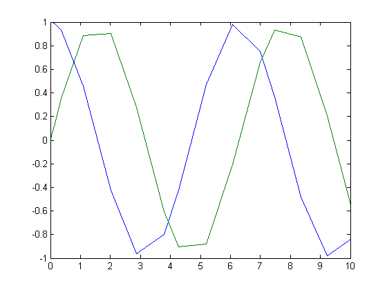
Add options.
options = odeset('MaxStep', 0.1, 'InitialStep', 0.05);
[t, x] = rkadapt(@(t,x) [-x(2); x(1)], [0 10], [1; 0], options);
plot(t, x);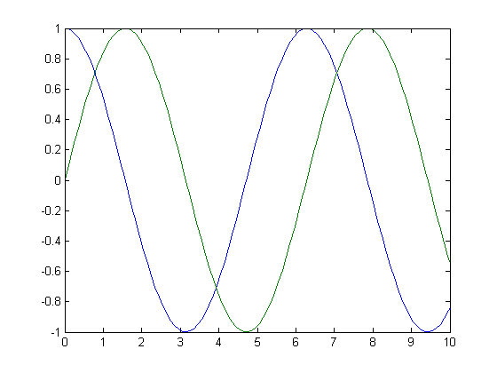
Now simulate with Bogacki-Shampine 3(2).
a = [  0   0   0 0; ...
     1/2   0   0 0; ...
       0 3/4   0 0; ...
     2/9 1/3 4/9 0];
b = [ 2/9 1/3 4/9   0; ... % For the update
     7/24 1/4 1/3 1/8];    % For the error prediction
c = [0 1/2 3/4 1];
p = 2;                     % The lower of the two orders
[t, x] = rkadapt(@(t,x) [-x(2); x(1)], [0 10], [1; 0], [], a, b, c, p);
plot(t, x);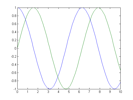
See Runge-Kutta methods on Wikipedia for discussion of the Butcher tableau (a, b, and c).
Reference
Dormand, J. R., and P. J. Prince. “A family of embedded Ruge-Kutta formulae.” Journal of Computational and Applied Mathematics 6.1 (1980): 19-26. Web. 22 Apr. 2014.
See Also
Solvers,odehybrid, rk4, rkfixed, ode45 (MATLAB), odeset (MATLAB)February 4th, 2023
©2023 An Uncommon Lab