rkfixed | An Uncommon Lab

`rkfixed`

Explicit Runge-Kutta fixed-step integration using the specified weights, nodes, and Runge-Kutta matrix (or the Runge-Kutta 4th order "3/8" method by default).

Implements numerical propagation of an ordinary differential equation from some initial value over the desired range. This function is similar to MATLAB's variable-step ODE propagators (e.g., ode45), but uses a fixed step method. This is useful either when one knows an appropriate step size or when a process is interrupted frequently (ode45 and the similar functions in MATLAB will always make at least a certain number of steps between ts(1) and ts(2), which may be very many more than are necessary).

This function is generic for all explicit fixed-step Runge-Kutta methods. That is, any explicit fixed-step Runge-Kutta propagator can be created by passing the weights, nodes, and Runge-Kutta matrix (together, the Butcher tableau) into this function. See the example below.

[t, x] = rkfixed(ode, ts, x0, dt);
[t, x] = rkfixed(ode, ts, x0, dt, a, b, c);
[t, x] = rkfixed(ode, ts, x0, options);
[t, x] = rkfixed(ode, ts, x0, options, a, b, c);

Inputs

ode	Ordinary differential equation function
ts	Time span, `[t_start, t_end]`
x0	Initial state (column vector)
dt	Time step
options	Alternately, one can specify an options structure instead of dt so that this function is compatible with `ode45` and its ilk. The only valid fields are `MaxStep` (the time step) and `OutputFcn`
a	Runge-Kutta matrix
b	Weights
c	Nodes

Outputs

t	Time history
x	State history, with each row containing the state corresponding to the time in the same row of `t`.

Example

Simulate an undamped harmonic oscillator for 10s with a 0.1s time step, starting from an initial state of [1; 0] using RK 4th order integration (via the Butcher tableau specified by a, b, and c). This is exactly the same as the rk4 function.

a = [0   0   0 0; ...
     0.5 0   0 0; ...
     0   0.5 0 0; ...
     0   0   1 0];
b = [1 2 2 1]/6;
c = [0 0.5 0.5 1];
[t, x] = rkfixed(@(t,x) [-x(2); x(1)], [0 10], [1; 0], 0.1, a, b, c);
plot(t, x);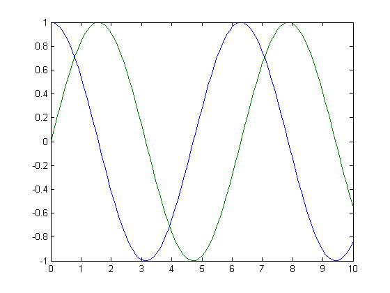

See Runge-Kutta methods on Wikipedia for discussion of the Butcher tableau (a, b, and c).

Docs

`rkfixed`

Inputs

Outputs

Example

See Also