by An Uncommon Lab

eif

Run one update of a basic extended information filter. Though less common than the extended Kalman filter, thi filter can be faster where the dimension of the measurement is larger than the dimension of the state, and has the advantage that it can start without any knowledge of the state, where the information matrix contains all zeros (corresponding to infinite covariance).

 x_k = F_km1 * x_km1 + G_km1 * w_q
 z_k = H_k * x_k + w_r

where km1 means k-1, w_q is a zero-mean Gaussian random variable with zero mean and covariance Q_km1. That is, w_q ~ N(0, Q_km1). Similarly, w_r ~ N(0, R_k).

It updates a state estimate and covariance from sample k-1 to sample k.

[x_k, Y_k] = eif(t_km1, t_k, x_km1, Y_km1, u_km1, z_k, ...
                 f, inv_F_km1, G_km1, inv_Q_km1, ...
                 h, H_k, inv_R_k);

Inputs

 x_k = f(t_km1, t_k, x_km1, u_km1);

 inv_F_km1 = fcn(t_km1, t_k, x_km1, u_km1)

 inv_Q_km1 = fcn(t_km1, t_k, x_km1, u_km1)

 x_k = f(t_km1, t_k, x_km1, u_km1);

 H_k = fcn(t_k, x_kkm1, u_km1)

 inv_H_k = fcn(t_k, x_k, u_km1)

Outputs:

Example

Similar to the example in the lkf function, we can quickly create a simulation for discrete, dynamic system, generate noisy measurements of the system over time, and pass these to an information filter.

First, define the discrete system.

rng(1);
dt    = 0.1;                                  % Time step
F_km1 = expm([0 1; -1 0]*dt);                 % State transition matrix
H_k   = [1 0];                                % Observation matrix
Q_km1 = 0.5^2;                                % Process noise variance
G_km1 = [0.5*dt^2; dt];                       % Process-noise-to-state map
R_k   = 0.1;                                  % Meas. noise covariance

Information filters work with inverses of many of these matrices (compared to Kalman filters).

inv_F = inv(F_km1);
inv_Q = inv(Q_km1);
inv_R = inv(R_k);

Make propagation and observation functions. These are just linear for this example, but eif would work fine with nonlinear functions.

f = @(t_km1, t_k, x_km1, u_km1) F_km1 * x_km1;
h = @(t_k, x_k, u_k) H_k * x_k;

Now, we'll define the simulation's time step and initial conditions. Note that we define the initial estimate and set the truth as a small error from the estimate (using the covariance).

n       = 100;                     % Number of samples to simulate
x_hat_0 = [1; 0];                  % Initial estimate
P       = diag([0.5 1].^2);        % Initial estimate covariance
Y       = inv(P);                  % Initial information matrix
x_0     = x_hat_0 + mnddraw(P, 1); % Initial true state

Now we'll just write a loop for the discrete simulation.

% Storage for time histories
x     = [x_0, zeros(2, n-1)];                         % True state
x_hat = [x_hat_0, zeros(2, n-1)];                     % Estimate
z     = [H_k * x_0 + mnddraw(R_k, 1), zeros(1, n-1)]; % Measurement
 
% Simulate each sample over time.
for k = 2:n
 
    % Propagate the true state.
    x(:, k) = F_km1 * x(:, k-1) + G_km1 * mnddraw(Q_km1, 1);
    
    % Create the real measurement at sample k.
    z(:, k) = H_k * x(:, k) + mnddraw(R_k, 1);
 
    % Run the Kalman correction.
    [x_hat(:,k), Y] = eif((k-1)*dt, k*dt, x_hat(:,k-1), Y, [], z(:,k), ...
                          f, inv_F, G_km1, inv_Q, h, H_k, inv_R);
 
end

Plot the results.

figure(1);
clf();
t = 0:dt:(n-1)*dt;
h = plot(t, x, ...
         t, z, '.', ...
         t, x_hat, '--');
legend('True x1', 'True x2', 'Meas.', 'Est. x1', 'Est. x2');
xlabel('Time');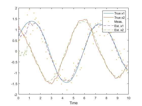

Note how similar this example is to the first example of lkf. The difference is the inverted matrices that this uses and the use of G_km1 with a 1-dimensional process noise which exactly matches the Q_km1 matrix used in the lkf example.

Reference

Bar-Shalom, Yaakov, X. Rong Li, and Thiagalingam Kirubarajan. Estimation with Applications to Tracking and Navigation. New York: John Wiley & Sons, Inc., 2001. Print. Pages 303-306.

See Also

lkf