Mr. Eustace's Jump: *kf Frameworks Tutorial

In October of 2014, Mr. Alan Eustace jumped from a balloon in the statosphere, broke the sound barrier in the thin atmosphere, fell for four minutes, deployed a parachute at 10,000 feet, and came to a gentle stop on the ground about ten minutes later. Let's suppose we were invited to watch this fantastic event and wanted to track Mr. Eustace's downward progress from the jump to the point that he deployed his chute. We'll use kff to build a series of Kalman filters, first generic, and then getting progressively better, and we'll see how well we track with a series of simulations.

But first, to see Mr. Eustace recount the trip and his team, you can see his TED talk here.

Going back to our example, here's what we have to work with:

We know the approximate position of the starting point of his jump, but not very accurately.
We have a telescope that our friend will use to track him over time, and the telescope automatically reads out its inclination angle to our computer. These measurements are also not very accurate.
We know nothing of the air currents which will push Mr. Eustace around, but certainly this will occur.
Oddly, Mr. Eustace and the world are 2-dimensional; we'll use positions as [rightward; upward] relative to the telescope with units of meters and meters/second.

Notice that the only measurement we have is an angle, which of course is insufficient to determine position by itself, but using this, combined with the approximately known dynamics, we'll be able to determine his position and velocity over time.

If you have *kf installed, you can follow along with this tutorial:

skfexample('eustace');

This will copy the example files into your local directory.

Problem Statement

Since we already know what sensors we'll have, our work begins by selecting a representation for the state. We'll keep this simple and use his position and velocity relative to the telescope, because it's easy to describe how this changes over time (force to acceleration to velocity to position) and how it becomes the measurement of the telescope's inclination angle (simple trigonometry). So let's define our state, $X$, as his position, $\vec{x}$, and velocity, $\dot{\vec{x}}$: $$X = \begin{bmatrix} \vec{x} \\ \dot{\vec{x}} \end{bmatrix} $$

To describe how this state changes over time, we note that his acceleration, $\ddot{\vec{x}}$, is governed by gravity and drag: $$\ddot{\vec{x}} = \vec{g} + \frac{1}{m} \vec{F}_d + \vec{F}_w$$

where $\vec{g}$ is gravity, $\vec{F}_w$ is some unknown wind force, and the drag force, $\vec{F}_d$, is: $$\vec{F}_d = -\frac{1}{2} c_d a \rho \|\dot{\vec{x}}\| \dot{\vec{x}}$$

where $c_d$ is the drag coefficient, $a$ is his area facing the direction of travel, $\rho$ is the air density, and $\dot{\vec{x}}$ is his velocity.

The propagation function is implemented in propagate_skydiver.m. It's interface is:

 x_k = propagate_skydiver(t_km1, t_k, x_km1, u_km1)

where t_km1 and t_k are the times at the last sample and current sample, respectively, x_km1 is the state (or estimate) at the last sample, and u_km1 is an input vector (which we don't use), and x_k is the update state (or estimate). This is the interface expected kff (though there can be additional inputs too; see the doc for kff).

The observation models are fairly simple. If his position relative to the telescope is $x$ in a [right; up] frame, then the elevation angle of the telescope that tracks him will be given by: $$\theta = \arctan\left( \frac{x_2}{x_1} \right) + \nu_\theta$$

where $\nu_\theta$ is random, momentary error.

The observation function is so simple in fact that we don't need to write a separate function for it and will use an anonymous function instead:

% Observation function
h = @(t_k, x_k, u_km1) ...
        atan2(x_k(2), x_k(1));

Again, we use the interface that kff expects for observation-related functions, which is the current time, current state, and current input vector (and we don't use an input vector, so we ignore it).

With these models, we can quickly make an extedned Kalman filter to track his progress, but that means, of course, that we'll also need the Jacobians.

Jacobians

Building a Kalman filter means we need to take the Jacobians of the dynamics and observation functions — the partial derivatives with respect to (wrt) the state. Though straight-forward, the Jacobian of the propagation function is tedious, so the actual derivation is in an appendix below. We have the implementation in propagation_jacobian.m, where the interface is the same as for the propgation function, namely:

F_km1 = propagation_jacobian([t_km1 t_k], x_km1, u_km1);

where F_km1 is the Jacobian at sample k-1.

Fortunately, the Jacobian of the observation function wrt the state is quite easy and can be implemented here as an anonymous function. $$\frac{\partial}{\partial X} \arctan\frac{x_2}{x_1} = \begin{bmatrix} \frac{-x_2}{x_1^2 + x_2^2} & \frac{x_1}{x_1^2 + x_2^2} & 0 & 0 \end{bmatrix} $$

% Function to calculate the Jacobian of the observation function
H_fcn = @(t_k, x_k, u_km1) ...
            [[-x_k(2), x_k(1)] ./ (x_k(1)^2 + x_k(2)^2), 0, 0];

Whenever we write functions to produce partial derivatives, we should test them to make sure they agree with an empirically-determined partial derivative of the underlying function, here f and h. The empirical determination is formed by evaluating $f$ at some state and then at several small perturbations from that state. Let's make sure our Jacobians look reasonable for some arbitrary state vector. To do this, we'll use *kf's built-in fdiff function, which takes in a function handle, a scalar or vector $\Delta X$ to use to create $X + \Delta X$, the input arguments to the propagation function, and an index to say which of those arguments is the state. (See fdiff for more.)

% We'll use this arbitrary state for testing [m; m; m/s; m/s].
x_test = [1000; 10000; 10; -200];
 
% We'll use this time step [s] throughout.
dt = 1;
 
% Calculate the Jacobian directly.
propagation_jacobian(0, dt, x_test)
 
% Empirically determine the partial derivative.
fdiff(@propagate_skydiver, 1e-6, 3, 0, dt, x_test)

ans =
    1.0000    0.0001    0.8673    0.0055
         0    0.9970    0.0055    0.7573
         0    0.0003    0.7469    0.0095
         0   -0.0055    0.0094    0.5565
ans =
    1.0000    0.0002    0.8540    0.0073
         0    0.9964    0.0073    0.7091
         0    0.0002    0.7768    0.0074
         0   -0.0039    0.0072    0.6244

Those agree pretty well, so our propagation_jacobian function is probably useable. (The differences are due to the nonlinearities of the propagation function compared to the linearizing assumptiong we make in order to calculate the Jacobian. A smaller dt would certainly bring the error down.)

How about for the observation Jacobian?

% Calculate the Jacobian directly.
H_fcn(0, x_test)
 
% Empirically determine the partial derivative.
fdiff(h, 0.001, 2, 0, x_test)

ans =
   1.0e-04 *
   -0.9901    0.0990         0         0
ans =
   1.0e-04 *
   -0.9901    0.0990         0         0

Perfect. We could test with more points, but we'll move on.

Process and Measurement Noise

We now need to specify what types of noise act on the system. For the process noise -- the random wind force mentioned above -- we'll suppose that there are random changes in wind that accelerate the skydiver both left-right and up-down. For the sake of the example, we can suppose that this is 1 m/s^2 in each axis (unrelated to the velocity, for the sake of simplicity). Mapping acceleration to a change in position and velocity, we'll have: $$Q = \begin{bmatrix} \frac{1}{4} \Delta t^4 & 0 & \frac{1}{2} \Delta t^3 & 0 \\ 0 & \frac{1}{4} \Delta t^4 & 0 & \frac{1}{2} \Delta t^3 \\ \frac{1}{2} \Delta t^3 & 0 & \Delta t^2 & 0 \\ 0 & \frac{1}{2} \Delta t^3 & 0 & \Delta t^2 \\ \end{bmatrix} q^2$$

where $q$ is the standard deviation of the acceleration noise (1 m/s^2).

q_accel = 1^2 * eye(2);                       % 1 m/s^2 std. dev.
G       = [0.5 * dt^2 * eye(2); dt * eye(2)]; % Maps accel. to state change
Q       = G * q_accel * G.';                  % Process noise covariance

The measurement noise is very easy. We'll suppose our inclinometer on the telescope has an error of 3 degrees, standard deviation. The variance (in radians^2) is thus:

R = (3 * pi/180)^2;

The First Simulation

Ok, we're now done describing the problem and can begin to use the Kalman filter framework. We'll build a simulation and call kff to filter on each step, using the matrices and functions from above. Let's initialize things.

% Set the random number generator seed so we can repeat this run.
rng(1);
 
% Set the initial estimate, uncertainty, and true state. The true state
% will be displaced from the estimate by some random draw according to P_0.
x_hat_0 = [5000; 41419; 100; 0];
P_0     = diag([1000 1000 20 20].^2); % 1km^2 pos. error; 20m/s vel. error
x_0     = x_hat_0 + mnddraw(P_0);

The easiest way to work with kff is to use the kffoptions structure and fill in the problem's functions and constants.

% Set up the KFF options with our functions and constants.
options = kffoptions('f',         @propagate_skydiver, ...
                     'h',         h, ...
                     'F_km1_fcn', @propagation_jacobian, ...
                     'Q_km1_fcn', Q, ...
                     'H_k_fcn',   H_fcn, ...
                     'R_k_fcn',   R);

Note that all of those matrices can be either function handles or constant values. If they're function handles, they'll be evaluated when they're needed. Otherwise, it will use the constant values for all time steps.

We can create the array of each time step and preallocate space for the true state over time, the estimate, the covariance, etc.

% Simulation end time, number of steps, and time history
t_end = 267; % 4m27s, the length of his fall
n     = ceil(t_end/dt);
t     = (0:n-1)*dt;
 
% Preallocate storage space.
x      = [x_0, zeros(4, n-1)];          % True states
z_true = zeros(size(R, 1), n);          % Perfect (noiseless) observations
x_hat  = [x_hat_0, zeros(4, n-1)];      % Estimated states
P      = cat(3, P_0, zeros(4, 4, n-1)); % Filter covariance
z      = zeros(size(R, 1), n);          % Measurements
z_hat  = zeros(size(R, 1), n);          % Filtered measurements

Now we'll implement the simulation loop. We'll use this loop again and again throughout this tutorial.

% Simulate.
rng(2); % We'll always seed with 2 before a single sim (apples to apples).
for k = 2:n
    
    % Propagate the real system (with noise).
    x(:,k) = propagate_skydiver(t(k-1), t(k), x(:,k-1)) + mnddraw(Q);
    
    % Make the "perfect" measurement, only for comparison later.
    z_true(:,k) = h(t(k), x(:,k));
 
    % Make the noisy measurement.
    z(:,k) = z_true(:,k) + mnddraw(R);
    
    % Run the filter.
    [x_hat(:,k), P(:,:,k)] = kff(t(k-1), t(k), x_hat(:,k-1), P(:,:,k-1),...
                                 z(:,k), options);
    
    % Also, log the predicted observation, for comparison later.
    z_hat(:,k) = h(t(k), x_hat(:,k));
    
end

That's it. On the whole, how well did we track?

% Calculate the estimation errors and display the mean errors.
err = x - x_hat;
fprintf('Performance of a single run of the extended Kalman filter:\n');
fprintf('Average position error: %.0f m\n',   ...
        mean(sqrt(sum(err(1:2,:).^2, 1))));
fprintf('Average velocity error: %.1f m/s\n', ...
        mean(sqrt(sum(err(3:4,:).^2, 1))));

Performance of a single run of the extended Kalman filter:
Average position error: 363 m
Average velocity error: 7.1 m/s

Let's plot the true trajectory and overlay the estimated trajectory.

% Trajectory
figure(1);
clf();
plot(x(1,:),     x(2,:),     '-', ...
     x_hat(1,:), x_hat(2,:), '--', ...
     [0 30000],  3048 * [1 1], 'r:');
xlabel('Downrange'); ylabel('Up');
axis equal;
axis([0 30000 0 45000]);
legend('True', 'Estimated', 'Chute Deploy');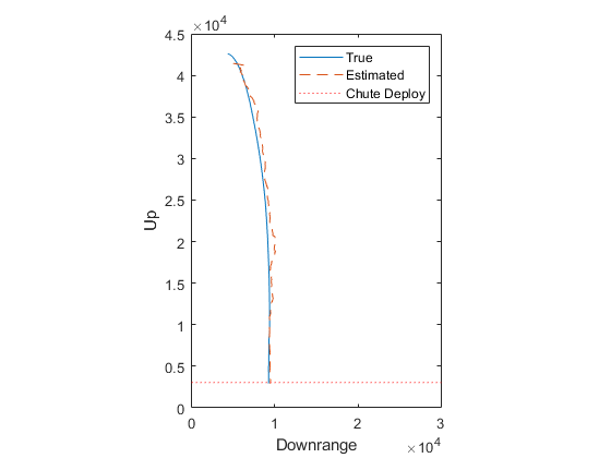

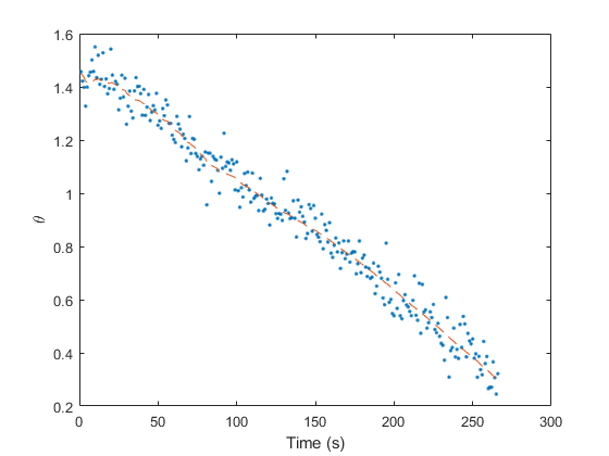
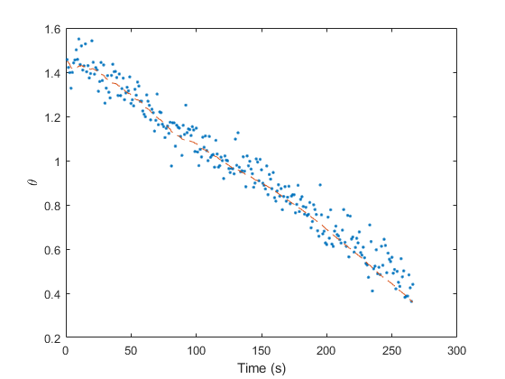
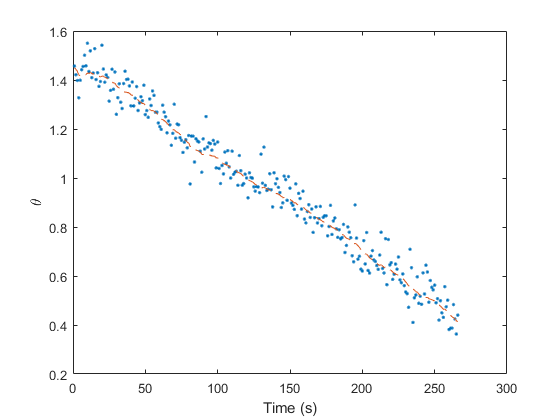
Similarly, let's plot the real measurements and the filtered measurements. To obtain the “filtered measurement” for sample k, we use the updated estimate for that sample and determine the expected value of the measurement — an estimate of what a noiseless measurement would be. If we've done a good job, it should run right down the middle of all of those noisy measurements.

% Observations
figure(2);
clf();
plot(t(2:end), z(1, 2:end), '.', ...
     t(2:end), z_hat(1, 2:end), '--')
xlabel('Time (s)'); ylabel('\theta');
legend('Measured', 'Filtered Measurement');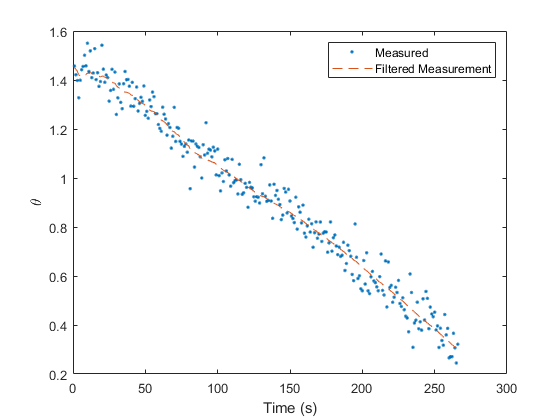

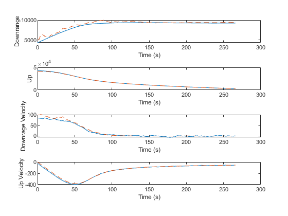
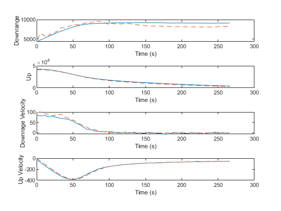
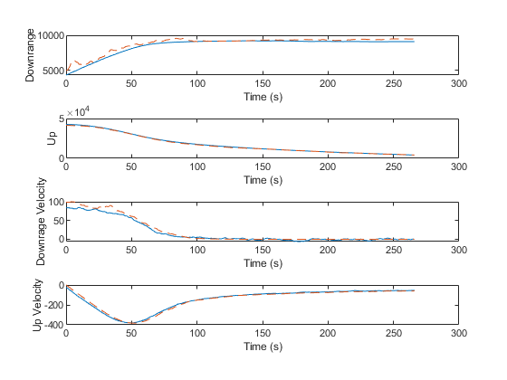
We can also plot every true state with the corresponding estimate.

% Line plots
figure(3);
clf();
subplot(4 ,1, 1);
plot(t, x(1, :),     '-', ...
     t, x_hat(1, :), '--');
xlabel('Time (s)'); ylabel('Downrange');
legend('True', 'Estimated');
subplot(4, 1, 2);
plot(t, x(2, :),     '-', ...
     t, x_hat(2, :), '--');
xlabel('Time (s)'); ylabel('Up');
subplot(4, 1, 3);
plot(t, x(3, :),     '-', ...
     t, x_hat(3, :), '--');
xlabel('Time (s)'); ylabel('Downrage Velocity');
subplot(4, 1, 4);
plot(t, x(4, :),      '-', ...
     t, x_hat(4, :), '--');
xlabel('Time (s)'); ylabel('Up Velocity');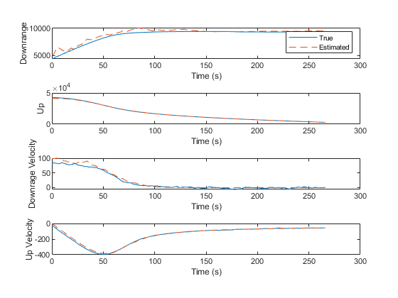

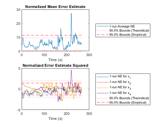
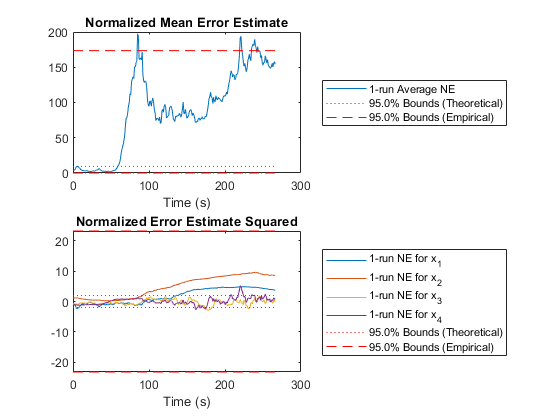
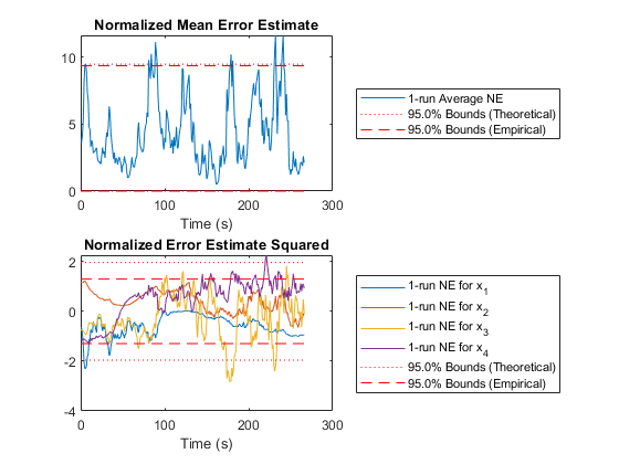
In the above plots, we can intuitively see how well we're filtering, but we don't know anything about the statistical properties. Here, we'll look at two plots of the estimate error (truth minus estimate) for each sample compared to the covariance matrix for each sample. We'll discuss NMEE and NEES more below, but basically, we're hoping to see that 95% of the errors are within the 95% boundaries corresponding to the covariance matrix.

% Errors (NMEE and NEES)
figure(4);
clf();
subplot(2, 1, 1);
normerr(err, P, 0.95, 1, 'XData', t, 'OneSided', true);
title('Normalized Mean Error Estimate');
xlabel('Time (s)');
subplot(2, 1, 2);
normerr(err, P, 0.95, 2, 'XData', t);
title('Normalized Error Estimate Squared');
xlabel('Time (s)');

Percent of data in theoretical 95.0% bounds: 89.9%
Percent of data in theoretical 95.0% bounds: 96.5%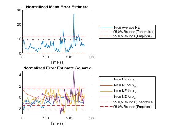

In fact, our results are pretty good.

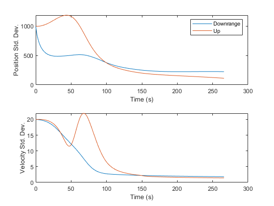
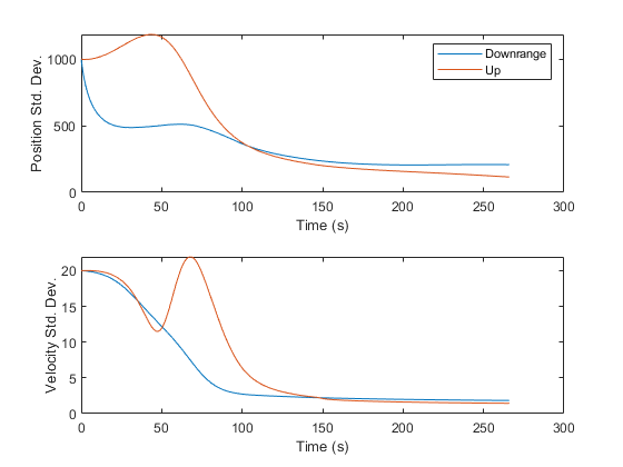
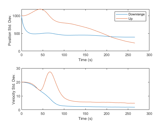
Finally, it's sometimes nice to see the error standard deviations, taken from the diagonals of the covariance matrix over time. This helps us see how much error we expect at each point along Mr. Eustace's freefall.

% Standard Deviations
figure(5);
clf();
subplot(2, 1, 1);
plot(t.', sqrt([squeeze(P(1,1,:)) squeeze(P(2,2,:))]));
xlabel('Time (s)'); ylabel('Position Std. Dev.');
legend('Downrange', 'Up');
subplot(2, 1, 2);
plot(t.', sqrt([squeeze(P(3,3,:)) squeeze(P(4,4,:))]));
xlabel('Time (s)'); ylabel('Velocity Std. Dev.');

It is interesting to see where the standard deviations increase and decrease. For instance, in the thin atmosphere, where drag matters little, we can extract very little information. However, as the air density and drag increase, the elements of the velocity are more strongly coupled, we can extract more information, and the covariance decreases. Then, as the skydiver approaches 10,000ft with a velocity more or less straight down, the angular measurements fail to provide much information about his downrange position, and uncertainty in that state levels off.

The results look fine, but how do we know if they're really good or bad? For starters, let's suppose we had merely propagated the initial position and velocity. How much error would we have in that case? We can plot it on top of our truth and estimate.

% Propagate the initial estimate without the filter.
x_hat_prop = [x_hat_0, zeros(4, n-1)];
z_hat_prop = zeros(size(R, 1), n);
for k = 2:n
    
    % Propagate and predict the observation.
    x_hat_prop(:,k) = propagate_skydiver(t(k-1), t(k), x_hat_prop(:,k-1));
    z_hat_prop(:,k) = h(t(k), x_hat_prop(:,k), []);
 
end
 
% Add the propagated position to the trajectory plot.
figure(1);
hold on;
plot(x_hat_prop(1, :), x_hat_prop(2, :), '-');
hold off;
legend('True', 'Estimated', 'Chute Deploy', 'Open-Loop');
 
% Add the open-loop predicted observations as well.
figure(2);
hold on;
plot(t(2:end), z_true(2:end), t(2:end), z_hat_prop(2:end));
hold off;
legend('Measured', 'Predicted', 'Perfect', 'Open-Loop');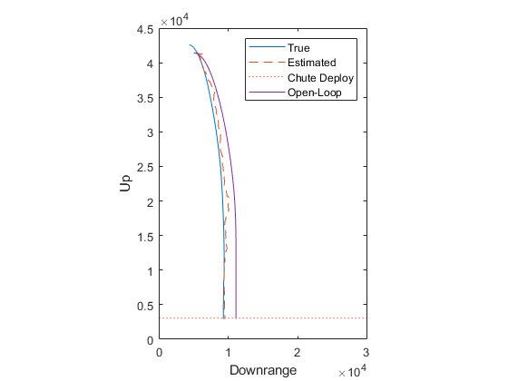

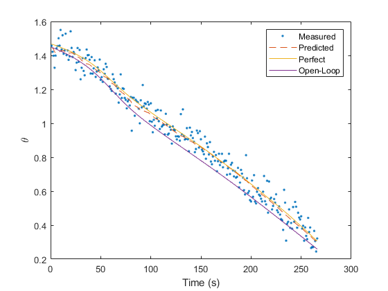
Obviously, our filter did much better than an open-loop propagation of our initial estimate.

Monte-Carlo Test of the Extended Kalman Filter

While the above error applies to this simulation, what if we'd taken different random draws? Do we expect to see similar performance all the time, or did we get lucky? There are many ways to answer this question, but one of the best is to run a Monte-Carlo test — a set of simulations starting from different initial conditions and proceding with different random draws throughout. Then, we can determine how well we can expect to estimate. Fortunately, when using the framework functions, this is trivial; we can call kffmct for “Kalman filter framework Monte-Carlo test” to do all of this for us, using the same kffoptions struct we've already been using for the filter. Let's have kffmct complete 20 runs from different real starting positions centered around our initial estimate, x_hat_0.

This will produce several statistics in the command window as well as several plots.

rng(3); % We'll always seed with 3 before a MCT (oranges to oranges).
[~, x, x_hat] = kffmct(20, ...      % Number of runs to perform
                    [0 t_end], ...  % Starting and ending times
                    dt, ...         % Time step
                    x_hat_0, ...    % Init. estimate to use for every run
                    P_0, ...        % Init. covariance to use for every run
                    options);       % kffoptions struct for our filter
 
% Print out the average position and velocity errors.
print_errors('MCT of the extended Kalman filter', x - x_hat);

NEES: Percent of data in theoretical 95.0% bounds: 85.8%
NMEE: Percent of data in theoretical 95.0% bounds: 98.0%
NIS:  Percent of data in theoretical 95.0% bounds: 95.5%
TAC:  Percent of data in theoretical 95.0% bounds: 94.4%
AC:   Percent of data in theoretical 95.0% bounds: 94.9%
Performance of a MCT of the extended Kalman filter:
Average position error: 616 m
Average velocity error: 9.2 m/s

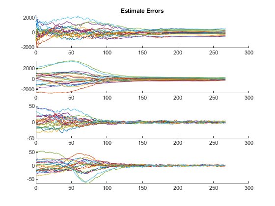
Some of those plots need some explanation.

The first figure shows the true states and estimates for all runs, right on top of each other.

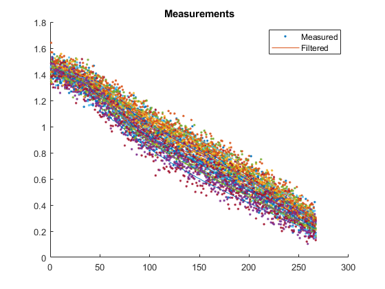
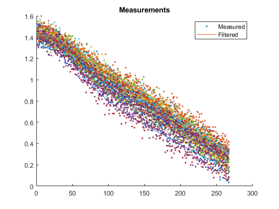
The next shows the measurements from each run along with the filtered measurements. To obtain the filtered measurements for a sample, we first run the filter with the corresponding, noisy measurement for that sample. Then, we use the new state estimate for that sample to determine what we would expect the measurement to be (we simply pass the updated state estimate to the observation function). This helps us to see how smooth our estimate is relative to the noisy measurements.

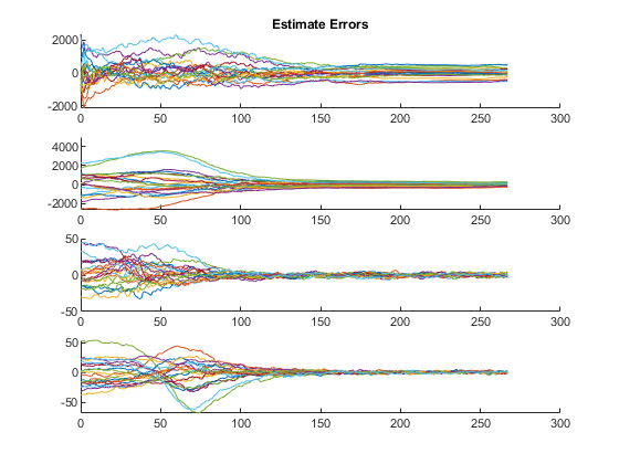
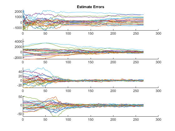
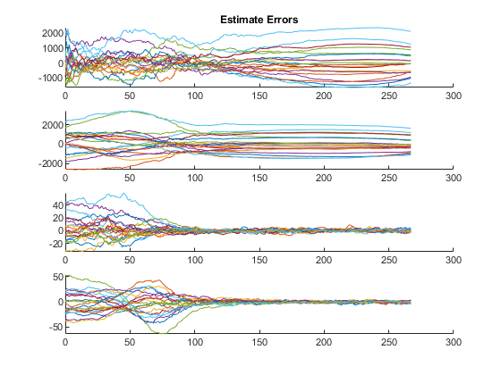
The third plot shows errors (truth minus estimates) for all of the states.

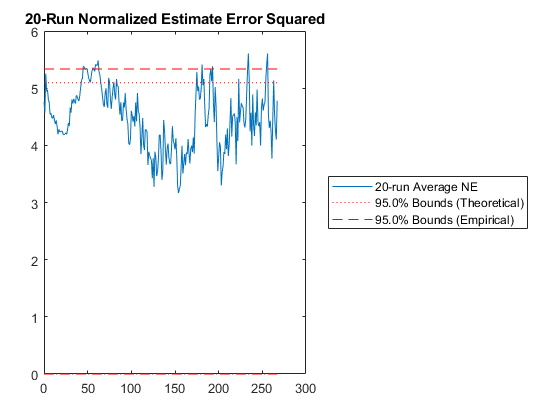
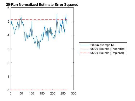
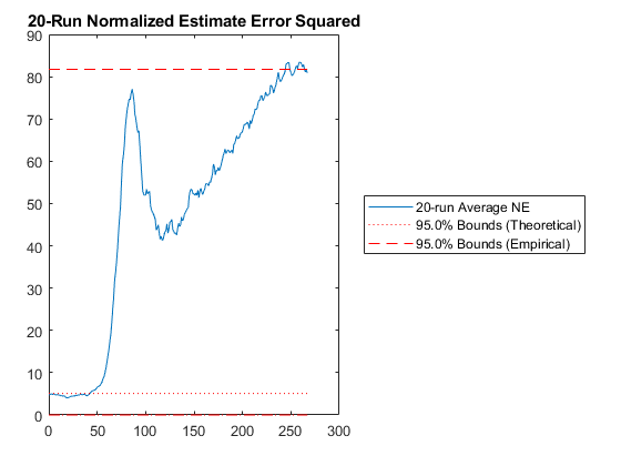
Then we have the n-run normalized estimation error squared (NEES). This is a powerful plot. It shows how well the filter performs relative to how well it “believes” it performs. For each sample and for each run, the true error is divided by the filter covariance for that sample: $$\left(x_k - \hat{x}_k\right)^T P_k^{-1} \left(x_k - \hat{x}_k\right)$$

The result is averaged across all runs. This should produce errors with a $\chi^2$ distribution. The 95% confidence bounds corresponding to the appropriate $\chi^2$ distribution are determined and shown on the plot as well. If the filter were performing exactly as expected, 95% of the real errors would be within the theoretical 95% confidence bounds. When more errors are within bounds, we can say that the filter is pessimistic -- it thinks it's doing worse than it is. When fewer errors are within bounds, we say that the filter is inconsistent with the filter assumptions and is optimistic -- it thinks it's doing better than it is. Optimism is particularly bad for extended Kalman filters, because it means that the errors might not correct fast enough, allowing the state estimate to wander, causing the Jacobians to be wrong, causing the state estimate to wander further. This is called divergence.

At what point should you be concerned? If only 92% of points are within the 95% bounds? 85%? 70%? For nonlinear problems, it's hard to pick a specific number. Regardless, as the number of runs are increased, the number should remain about the same. If the number decreases with increasing numbers of runs, then likely the estimate errors aren't zero-mean but instead have a bias, and the designer may need to spend time revising the filter until it's appropriately zero-mean.

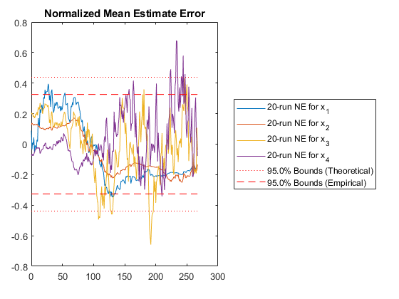
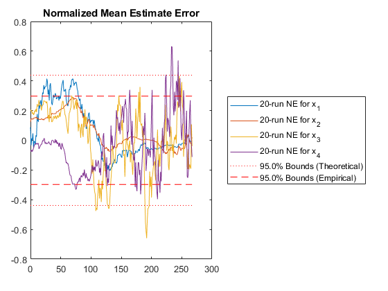
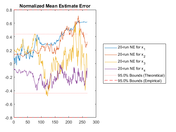
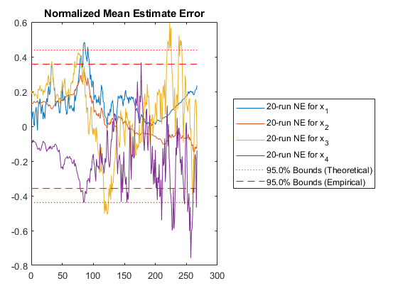
The fifth plot can be used in conjunction with the plot above, as it is another way of looking at errors relative to what's expected from the covariance. In this plot, we calculate the normalized mean estimate error (NMEE) for each element, $i$, of the state as: $$\left(x_{i,k} - \hat{x}_{i,k}\right) / \sqrt{P_{i,i,k}}$$

where $P_{i,i,k}$ is the $i$th diagonal of the covariance matrix for the $k$th sample and similarly $x_{i,k}$ is the $i$th element of the state/state estimate for sample $k$.

These errors are expected to be Gaussian, and corresponding bounds are determined. Again, we expect 95% of the errors to be within the 95% confidence bounds predicted by the covariance matrix. When this is not so, it's easy to see in this plot which particular states may be the problem.

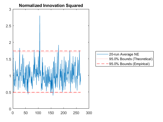
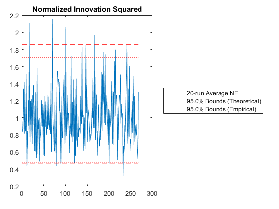
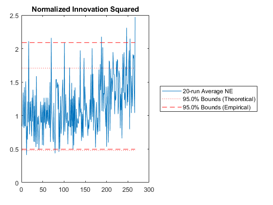
The sixth plot is exactly the same as the NEES plot, but instead of using the state error and covariance, it uses the innovation vector (measurement minus predicted measurement) and its covariance. It's called the Normalized Innovation Squared.

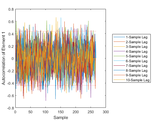
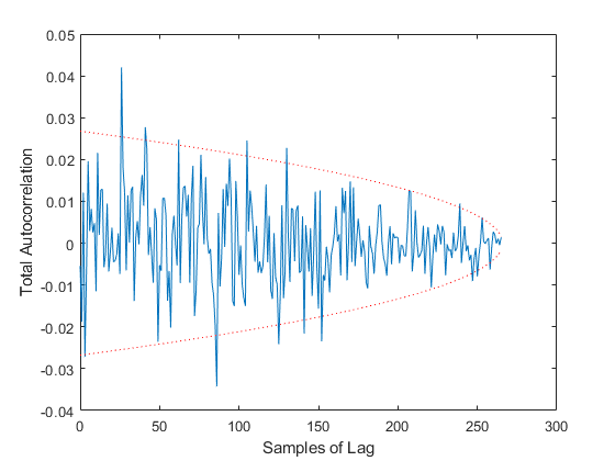
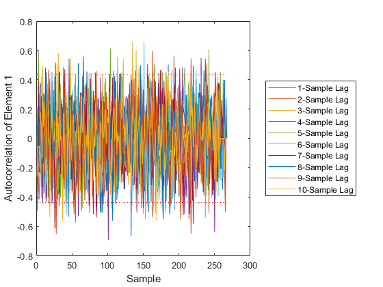
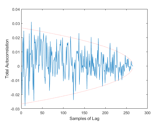
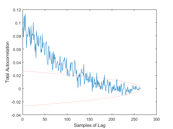
Finally, we have two tests of autocorrelation in the innovation vector. One shows the overall autocorrelation for every possible number of samples of lag, along with the associated 95% bounds. If the autocorrelation is outside of these bounds for more than 95% of the samples, then we have reason to believe that our errors are not white, but that errors at one point in time predict to some degree later errors. This would suggest that we aren't taking advantage of the observations well, perhaps in our modeling of the Jacobian or measurement noise covariance matrix.

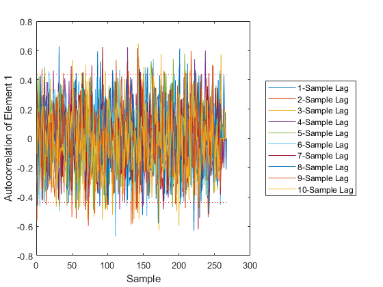
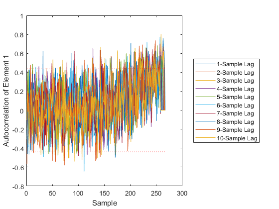
The final plot shows the autocorrelation over time of individual elements at various numbers of samples of lag. It can help identify which element of the measurement we are not predicting well.

All of the statistics are printed to the command window as well.

In our case, these plots seem to indicate that we're doing a reasonbly good job, at least given our simulation so far.

An Iterated Extended Kalman Filter

Our performance is pretty good compared to our awful measurements, but perhaps we can do a little better. The ability for a Kalman filter to correct the estimate over time is tied largely to how well those Jacobians match reality. A Kalman filter is only optimal when those Jacobians exactly match the truth. Since we don't know reality, we use the estimated state to determine the Jacobians. However, as soon as we've run the Kalman filter, then we have a better estimate, which we could use to create a better Jacobian, which we could then use to re-correct our predictions. Of course, this process could repeat until the Jacobian converged sufficiently to (hopefully) the true value. Filters employing this technique are called iterated extended filters.

Adding iteration to a kff filter is trivial. We can simply ask for it in the options struct. It's a one-line change.

% This is the number of times the observation Jacobian will be calculated;
% using 1 corresponds to a regular extended filter; anything more than one
% is an iterated extended filter. We'll use 2 for a single correction to
% the observation Jacobian.
options.num_iterations = 2;

With that additional option in place, here is our simulation again. This time, all of the plots have been wrapped up in plot_results.m.

% Simulate
rng(2);
x     = [x_0, zeros(4, n-1)];
x_hat = [x_hat_0, zeros(4, n-1)];
P     = cat(3, P_0, zeros(4, 4, n-1));
z     = zeros(size(R, 1), n);
z_hat = zeros(size(R, 1), n);
for k = 2:n
    
    % Propagate the real system (with noise).
    x(:,k) = propagate_skydiver(t(k-1), t(k), x(:,k-1)) + mnddraw(Q);
    
    % Make the measurement.
    z(:,k) = h(t(k), x(:,k)) + mnddraw(R);
    
    % Run the filter.
    [x_hat(:,k), P(:,:,k)] = kff(t(k-1), t(k), x_hat(:,k-1), P(:,:,k-1),...
                                 z(:,k), options);
    
    % Also, log the predicted observation, for comparison later.
    z_hat(:,k) = h(t(k), x_hat(:,k));
    
end
 
% Plot the results.
fprintf(['Performance of a single run of the iterated extended ' ...
         'Kalman filter:\n']);
plot_results(t, x, z, x_hat, z_hat, P);

Performance of a single run of the iterated extended Kalman filter:
Average position error: 346 m
Average velocity error: 7.1 m/s
Percent of data in theoretical 95.0% bounds: 88.4%
Percent of data in theoretical 95.0% bounds: 96.6%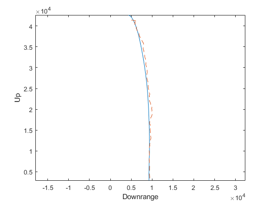

This seems like a nice improvement. By changing a single value, we've improved our estimate by about 40m.

Iteration affects the calculation of the observation-related matrices only (H and R). It doesn't effect propagation (F or Q), because the propagation matrices were already calculated based on the last corrected value. (However, there is such as thing as “going back in time” to re-estimate old information, like the last few estimates, using the new measurement. This is called smoothing, but we leave the discusssion of this for another day.)

Let's run another Monte-Carlo test to see what improvement we can expect overall.

rng(3);
[~, x, x_hat] = kffmct(20, [0 t_end], dt, x_hat_0, P_0, options);
 
% Print out the average position and velocity errors.
print_errors('MCT of the iterated extended Kalman filter', x - x_hat);

NEES: Percent of data in theoretical 95.0% bounds: 84.0%
NMEE: Percent of data in theoretical 95.0% bounds: 98.3%
NIS:  Percent of data in theoretical 95.0% bounds: 95.5%
TAC:  Percent of data in theoretical 95.0% bounds: 94.4%
AC:   Percent of data in theoretical 95.0% bounds: 94.8%
Performance of a MCT of the iterated extended Kalman filter:
Average position error: 610 m
Average velocity error: 9.2 m/s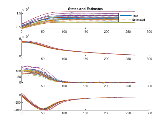

Hm, without iteration, we had about 420m of error, but with iteration we have 410m. It's not much improvement. The Monte-Carlo testing has revealed that iteration is in fact not helping us much. However, since we're unconcerned with the extra time required to run the filter, we'll leave iteration in place as we go forward.

Uncertainty in the Air Density and Drag Coefficient

Up to this point, we've been using the same models for the propagation of the estimate as we have for the propagation of the true state, but of course we are rarely able to model reality quite so well. For instance, the atmosphere is certainly not the same every day. Pilots have to adjust their altimeters with the barometric pressure offset of the area they're flying over. Further, no matter how many experiments we've run, we probably don't have great certainty of the effective drag coefficient, $c_d$.

Let's include these errors this in our model. For the air density discrepancy, we'll use a height offset at the ground corresponding to an air density offset. So, in the real propagation, the air density, $\rho$, will be calculated as: $$\rho = f(h_{true} + h_{offset})$$

whereas in our model, we'll continue to use: $$\rho_{estimated} = f(h_{estimated})$$

without any knowledge of the height offset. (Yes, we could measure the barometric pressure at the ground, but let's say we left the pressure gauge at home so that we can see what will happen.)

Further, we'll propagate with a slightly wrong value for $c_d$.

To do this, we'll keep using the same simulation loop, this time only changing the propagation of the truth to use propagate_skydiver_offset, which has the erroneous values in it.

% Simulate
rng(2);
x     = [x_0, zeros(4, n-1)];
x_hat = [x_hat_0, zeros(4, n-1)];
P     = cat(3, P_0, zeros(4, 4, n-1));
z     = zeros(size(R, 1), n);
z_hat = zeros(size(R, 1), n);
for k = 2:n
    
    % Propagate the real system (with noise).
    x(:,k) =   propagate_skydiver_offset(t(k-1), t(k), x(:,k-1)) ...
             + mnddraw(Q);
    
    % Make the measurement.
    z(:,k) = h(t(k), x(:,k)) + mnddraw(R);
    
    % Run the filter.
    [x_hat(:,k), P(:,:,k)] = kff(t(k-1), t(k), x_hat(:,k-1), P(:,:,k-1),...
                                 z(:,k), options);
    
    % Also, log the predicted observation, for comparison later.
    z_hat(:,k) = h(t(k), x_hat(:,k));
    
end
 
% Plot the results.
fprintf('Performance of a single run with model mismatch:\n');
plot_results(t, x, z, x_hat, z_hat, P);

Performance of a single run with model mismatch:
Average position error: 1237 m
Average velocity error: 7.9 m/s
Percent of data in theoretical 95.0% bounds: 21.7%
Percent of data in theoretical 95.0% bounds: 67.9%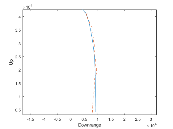

The estimate tracks reasonably well up high, where the difference in height makes only a small difference in air density and the density is so low that drag doesn't matter as much, but the problem is pronounced down low. Further, our filter's covariance does not “know” about this error source at all, and so far more errors lie outside of the 95% confidence bounds. This makes our filter inconsistent, with estimates liable to wander off with nonetheless great confidence that they're tracking. This is bad, so how can we consider the effect of this additional model uncertainty?

Upon first consideration, it may be tempting to use Q. It is, after all, the representation of unknown noise in the propagation, and we could think of the error in the air density and drag coefficient as unknown noise. However, how would this reflect the way the air density error maps to the state change? It largely wouldn't. Instead, we can treat the height offset and drag coefficient as consider parameters with associated consider covariance. We can find the Jacobian of the propagation function wrt these consider parameters, and then we'll pass all of this to kff, which will incorporate the additional uncertainty and use it intelligently to correct the state, making a Schmidt-Kalman filter. Let's see how.

First, we need to determine what the covariance of the height offset and drag coefficient are. For this example, we'll say they're +/- 500m standard deviation and 0.2 standard deviation. This is our consider covariance matrix.

P_cc = [500^2, 0; 0, 0.2^2]; % Consider covariance matrix

Next, we determine the mapping of these parameters to the dynamics — that is, the Jacobian of the propagation function wrt the height offset and drag coefficient. We have this implemented in propagation_jacobian_consider.m, with the same interface as before:

F_c_km1 = propagation_jacobian_consider([t_km1 t_k], x_km1, u_km1);

where F_c_km1 is the Jacobian wrt the consider parameters at sample k-1.

We must do the same for the observation function, but it doesn't depend on the air density or drag coefficient, so it's just a couple of zeros (the dimension of the measurement, 1, by the number of consider parameters, 2).

Hc = [0, 0];

We'll need one more thing to create the consider filter: the initial covariance between the state estimate and the consider parameters. We'll say there's no initial covariance between state errors and consider parameter errors, a reasonable assumption here.

P_xc_0 = zeros(4, 2); % number of states by number of consider parameters

We're ready to simulate again. Note the two additional terms in kffoptions.

options = kffoptions('f',               @propagate_skydiver, ...
                     'h',               h, ...
                     'F_km1_fcn',       @propagation_jacobian, ...
                     'Q_km1_fcn',       Q, ...
                     'H_k_fcn',         H_fcn, ...
                     'R_k_fcn',         R, ...
                     'num_iterations',  2, ...
                     ... New consider stuff ...
                     'F_c_km1_fcn',     @propagation_jacobian_consider, ...
                     'H_c_k_fcn',       Hc, ...
                     'P_cc',            P_cc);
 
% Simulate
rng(2);
x     = [x_0, zeros(4, n-1)];
x_hat = [x_hat_0, zeros(4, n-1)];
P     = cat(3, P_0, zeros(4, 4, n-1));
P_xc  = cat(3, P_xc_0, zeros(4, 2, n-1)); % Note that this is new.
z     = zeros(size(R, 1), n);
z_hat = zeros(size(R, 1), n);
for k = 2:n
    
    % Propagate the real system (with noise).
    x(:,k) =   propagate_skydiver_offset(t(k-1), t(k), x(:,k-1)) ...
             + mnddraw(Q);
    
    % Make the measurement.
    z(:,k) = h(t(k), x(:,k)) + mnddraw(R);
    
    % Run the filter.
    [x_hat(:,k), P(:,:,k), P_xc(:,:,k)] = kff( ...
        t(k-1), t(k), x_hat(:,k-1), P(:,:,k-1), P_xc(:,:,k-1), ...
        [], z(:,k), options);
    
    % Also, log the predicted observation, for comparison later.
    z_hat(:,k) = h(t(k), x_hat(:,k));
    
end
 
% Plot the results.
fprintf('Performance of a single run with Schmidt-Kalman filter:\n');
plot_results(t, x, z, x_hat, z_hat, P);

Performance of a single run with Schmidt-Kalman filter:
Average position error: 518 m
Average velocity error: 9.7 m/s
Percent of data in theoretical 95.0% bounds: 95.5%
Percent of data in theoretical 95.0% bounds: 98.3%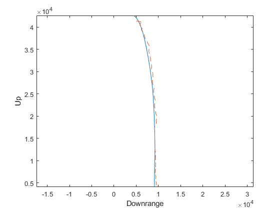

Our error is much reduced, from over 1km to 465m.

Despite that our truth simulation has a height offset of 450m and a drag coefficient 12.5% higher than the real value, which the estimator knows nothing about, the estimator's covariance is updated with the uncertainty in these parameters, and the true errors are within what's expected by the covariance. All we needed to do to transition from our iterated extended Kalman filter to an iterated extended Schmidt-Kalman filter was add in the two new Jacobians, define the consider covariance, and the state-consider covariance (P_xc) in our call to kff.

We've now handled a disagreement between the model and (simulated) reality. Let's try the same thing, but across many runs, each with different height offsets and drag coefficients, by calling kffmct with our additional consider matrices and functions, P_cc, F_c, and H_c. It will use P_cc to generate different consider parameter errors for each run and will use the Jacobians to map them to the true state update and measurement. With this one line, we have the simulation results of 20 different runs of our iterated extended Schmidt-Kalman filter.

rng(3);
[~, x, x_hat] = kffmct(20, [0 t_end], dt, x_hat_0, P_0, P_xc_0, [], options);
 
% Print out the average position and velocity errors.
print_errors('MCT of the Schmidt-Kalman filter', x - x_hat);

NEES: Percent of data in theoretical 95.0% bounds: 94.0%
NMEE: Percent of data in theoretical 95.0% bounds: 83.8%
NIS:  Percent of data in theoretical 95.0% bounds: 93.3%
TAC:  Percent of data in theoretical 95.0% bounds: 94.4%
AC:   Percent of data in theoretical 95.0% bounds: 95.0%
Performance of a MCT of the Schmidt-Kalman filter:
Average position error: 817 m
Average velocity error: 10.3 m/s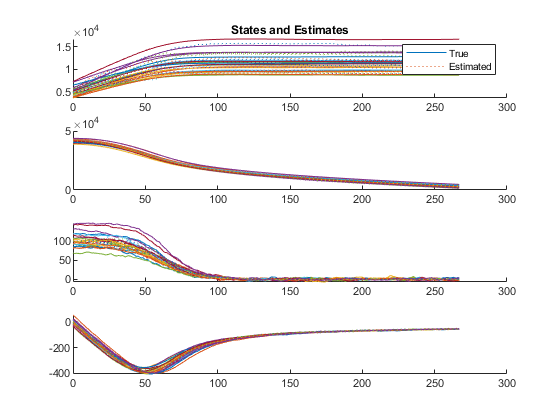

Our error is higher than before because now the truth simulation is more uncertainty in it. However, we're dealing with this appropriately in the filter, and our results are far better than they would be if we ignored the consider parameters in the filter. Of course, we can test this to show that it's true, which we do next.

Mismatched Model with `kffmct`

The above simulations include the consider parameter errors in the propagation of the truth, and our filter uses the consider covariance correctly. However, how bad would the Monte-Carlo test have gone if the simulation used the consider parameter errors, but the filter did not use the consider covariance? kffmct allows the true propagation and measurement functions to be different from those used by the filter. This is useful for making the simulation use a complex simulation while the filter uses a simpler model. In this case, we can take advantage of this to make sure the filter doesn't use consider covariance while the simulation does. We'll pass the full system definition to kffmct; this will be used for the simulation, but the options structure that defines the filter will have no mention of the consider parameters and will operate exactly the same as our iterated extended Kalman filter from several sections back.

options = kffoptions('f',               @propagate_skydiver, ...
                     'h',               h, ...
                     'F_km1_fcn',       @propagation_jacobian, ...
                     'Q_km1_fcn',       Q, ...
                     'H_k_fcn',         H_fcn, ...
                     'R_k_fcn',         R, ...
                     'num_iterations',  2); % No consider stuff here!
 
% Note that now we pass *everything* in to kffmct so that it can simulate
% with different values than those used by the filter via the options
% structure.
rng(3);
[~, x, x_hat] = kffmct(20, [0 t_end], dt, x_hat_0, P_0, P_xc_0, ...
                    @propagate_skydiver, ...
                    @propagation_jacobian_consider, ...
                    Q, ...
                    h, Hc, R, ...
                    P_cc, ...
                    options);
 
% Print out the average position and velocity errors.
print_errors('MCT of the mismatched models without consider covariance',...
             x - x_hat);

NEES: Percent of data in theoretical 95.0% bounds: 16.0%
NMEE: Percent of data in theoretical 95.0% bounds: 96.4%
NIS:  Percent of data in theoretical 95.0% bounds: 88.4%
TAC:  Percent of data in theoretical 95.0% bounds: 48.1%
AC:   Percent of data in theoretical 95.0% bounds: 89.6%
Performance of a MCT of the mismatched models without consider covariance:
Average position error: 1031 m
Average velocity error: 9.1 m/s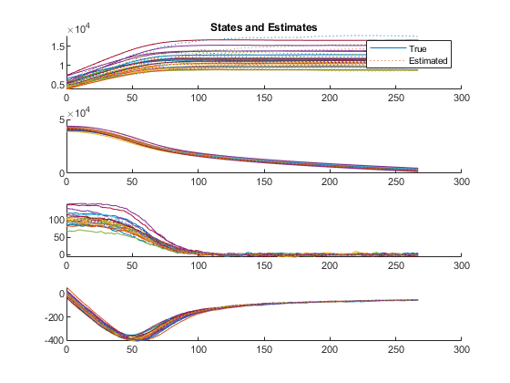

The difference is huge, hundreds of meters. Not only is the error large, but our filter is horribly inconsistent, with far too many errors ourside of the 95% confidence bounds and autocorrelation showing large biases. Clearly, if the real world has such variability in the air density and drag coefficients, then we need to include that uncertainty in our filter. The Schmidt-Kalman filter was in fact the right way to go.

Another option would have been to try to estimate the height offset and coefficient of drag directly, which we could have done for a small improvement. However, many serious filters need some amount of consider covariance, so it's good to know how to do it.

Summary

This brings us to the end of the tutorial. We've built an extended Kalman filter for a stratospheric skydiver, added iteration to the filter, and added discrepancies between the filter's propagation and the true propagation. Further, we've run Monte-Carlo tests of all of these cases and examined the statistical properties to determine how well we've ultimately done. However, we wrote no code for the various filters we tried and no code for the Monte-Carlo tests or the statistical analyses. We merely described our problem in several different ways and relied on the tools to explore the space of possible filters quickly and confidently.

Presumably, Mr. Eustace and his team had far better instruments tracking his fall (and presumably their models were 3-dimensional). However, their filtering techniques may well have been similar in scope to what we've explored here. How much more information could we have extracted from their real data? How well could we have known his position and velocity in real time if we had more than a noisy inclinometer? What other elements, like drag coefficient or orientation, would we want to estimate? How might we create a better drag model from what we've observed in order to track the next stratospheric jump? We don't answer these questions here, but point instead to Mr. Eustace's trek as something we might all like to know a little more about, and with the framework tools, we have many ways in which we might begin to explore.

Next Steps

From *kf, we used:

kff for the actual filtering,
kffoptions to specify what the filter should use and do,
kffmct to run Monte-Carlo tests of the filter, and
fdiff to make sure our Jacobian functions were working correctly.

Reading more on any of these would be a good next step for more information.

For a brief discussion of the Jacobian of the propagation function, see below.

Appendix: The Jacobian of the Propagation Function

Here, we show the math behind the Jacobian of the propagation function wrt the state. The state and dynamics are discussed above. Since the state is the position and velocity, the time-derivative of the state is velocity and acceleration. We have the acceleration defined in terms of the current velocity, gravity, drag, and wind noise terms, like so: $$\ddot{\vec{x}} = \vec{g} - \frac{1}{m} \frac{1}{2} c_d a \rho \|\dot{\vec{x}}\| \dot{\vec{x}} + \vec{F}_w$$

The Jacobian of the continuous-time dynamics function, $A$, is then: $$A = \begin{bmatrix} 0_{2x2} & 1_{2x2} \\ \frac{\partial}{\partial \vec{x}} \ddot{\vec{x}} & \frac{\partial}{\partial \dot{\vec{x}}} \ddot{\vec{x}} \\ \end{bmatrix}$$

where $1_{2x2}$ is a 2-by-2 identity matrix. We can expand the partial derivative of the acceleration wrt the position as: $$\frac{\partial}{\partial \vec{x}} \ddot{\vec{x}} = -\frac{1}{2} \frac{1}{m} c_d a \|\dot{\vec{x}}\| \begin{bmatrix} 0 & \dot{x}_1 \frac{\partial}{\partial x_2} \rho \\ 0 & \dot{x}_2 \frac{\partial}{\partial x_2} \rho \\ \end{bmatrix}$$

where $\frac{\partial}{\partial x_2} \rho$ can be calculated using a table-lookup. Of course, the acceleration does not depend at all on the downrange position component.

The partial derivative of the acceleration wrt the velocity is: $$\frac{\partial}{\partial \dot{\vec{x}}} \ddot{\vec{x}} = -\frac{1}{2} \frac{1}{m} c_d a \rho \left( \dot{\vec{x}} \dot{\vec{x}}^T \frac{1}{\|\dot{\vec{x}}\|} + \|\dot{\vec{x}}\| 1_{2x2} \right)$$

These can be verified for each scalar element of the Jacobian in a few minutes by using the product rule on the $\|\dot{\vec{x}}\| \dot{\vec{x}}$ terms.

Putting these together to form $A$, we have the Jacobian of the continuous-time dynamics. For a discrete filter, we'll need the Jacobian of the discrete-time dynamics. If we approximate $A$ as constant across a time step, then we can obtain the discrete Jacobian as: $$F = e^{A \Delta t}$$

where $\Delta t$ is the time step from discrete sample to discrete sample, and$e$ in this case is a matrix exponential, expm in MATLAB.

This is implemented in propagation_jacobian.m.

A similiar derivation is used for the Jacobian of the propagation function wrt the consider parameters.

Problem Statement
Jacobians
Process and Measurement Noise
The First Simulation
Monte-Carlo Test of the Extended Kalman Filter
An Iterated Extended Kalman Filter
Uncertainty in the Air Density and Drag Coefficient
Mismatched Model with kffmct
Summary
Next Steps
Appendix: The Jacobian of the Propagation Function

Docs